4-Transport

After generating particle paths and estimating ammonium and nitrate concentrations at the water table, the Transport Module (Figure 2‑14) estimates the plumes of ammonium and nitrate, i.e., the spatial distribution of their concentrations, using the Domenico solution’s steady state, 2D version. Note that the calculations performed by this module are the most computationally demanding out of all the modules. If there is insufficient memory or free disk space, calculations may fail unexpectedly. If this happens, users need to reduce the resolution or conduct the simulation for a sub-area of the domain. A common practice is to first split the OSTDS into several sub-areas, prepare corresponding OSTDS input files, and then run ArcNLET-Py for the input files. There is no need to re-do the flow and Particle Tracking Modules because the flow conditions do not change between the ArcNLET-Py runs. After the ArcNLET-Py runs, one can mosaic together the plumes generated by the runs.

The transport model is based on an analytical solution introduced by Domenico and Robbins (1985) for the advection-dispersion equations that govern the transport of ammonium and nitrate. This analytical solution considers advection along a single dimension and dispersion along one, two, or three dimensions. Additionally, it assumes homogenous flow fields and homogeneous aquifer transport properties. The advantage of using an analytical solution is that the concentration of contaminants can be determined anywhere, anytime, without having to solve any differential equations numerically. For more advanced solute transport modeling with complicated hydrogeological conditions (e.g., heterogeneous aquifer transport properties), one should use more sophisticated software and/or computer codes such as MT3DMS.

The Domenico solution used in this Python Toolbox is a two-dimensional, steady-state with first-order decay (first-order decay is used to simulate denitrification (Domenico, 1987)). This formulation produces a two-dimensional plume later converted to a pseudo-3D form by extending the 2D solution in the vertical dimension. Using a pseudo-3D form avoids the large memory requirements of calculating the complete 3D solution formulated by Domenico and Robbins (1985). The shape of each plume depends on the groundwater flow field near the NO₃ or NH₄ source, as determined by the Groundwater Flow Module. Since the analytical solution requires uniform flow to deal with heterogeneity in the flow magnitude, the harmonic mean averaged along the flow path is used. This average value is used in evaluating the analytical solution. Heterogeneous porosity is handled by averaging the porosity along the path using the arithmetic mean. Heterogeneous decay coefficients and dispersivities are handled using a constant value for each plume, with the possibility of the values varying from plume to plume. The values of the decay coefficient and dispersivities should be representative of the plume. Each plume is individually warped to conform to a flow path, using a first- or second-order transformation or a thin-plate spline transformation to handle curved paths.

Note that the Domenico solution is for a single species (i.e., ammonium or nitrate). Zhu et al. (2016) expanded the solution for both ammonium and nitrate with the transformation introduced by Sun et al. (1999). The current version of ArcNLET-Py is based on the work of Zhu et al. (2016).

The outputs of the Transport Module are a raster, representing the combined concentration distribution of all OSTDS, and an auxiliary point shapefile that stores associated plume information (e.g., transport simulation parameters, calculated mass inputs, etc.) for each OSTDS. Lastly, the plume info shapefile output from the Transport Module is used in the functionality of the Load Estimation Module to determine load from OSTDS to surficial water bodies.

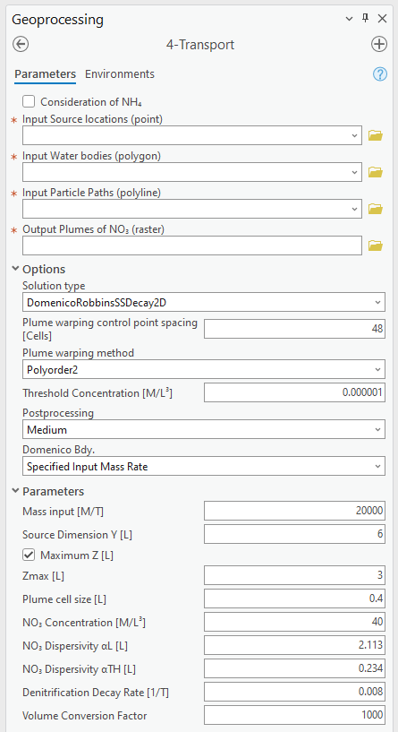
Figure 2‑14: The Transport Module.

Input Layers

• Consideration of NH4: This option allows for estimating the load of ammonium (NH₄⁺) to surface water bodies. By default, this option is unchecked. Utilizing this option increases computation time. There are several input fields revealed when considering NH₄⁺.

• Input Source locations (point): This layer specifies the areas of the contaminant sources. This point feature class may optionally contain several numeric (FLOAT) fields in its attribute table that allow for the specification of transport parameters on a source-by-source basis. The fields that are permitted are described in Table 2‑6.

Table 2‑6: Optional parameters in the attribute table of the source locations file.

Field Name	Description	**Corresponding Parameter**
no3_conc	The initial concentration of the source plane for nitrate-nitrogen.	C0 [M/l3]
nh4_conc	The initial concentration of the source plane for ammonium-nitrogen.	C0 [M/l3]

The field names must be labeled as shown in the table and be of the FLOAT type. If one wants to use constant concentrations of ammonium and/or nitrate for all OSTDS, he/she can input the concentration values in the Parameters section.

• Input Water bodies (polygon): Specifies the locations of water bodies. It is the same input used in the Particle Tracking Module.

• Input Particle Paths (polyline): The particle paths correspond with the Source locations and are the output file of the Particle Tracking Module. The Transport Module uses this file to calculate the average velocity (harmonic mean) and porosity (arithmetic mean) along each flow path. These values are then used for the calculation of each plume.

Options and Parameters

• Solution type: The form of the Domenico solution to use. The available options are:

1. DomenicoRobbinsSS2D: The two-dimensional, steady-state Domenico solution without decay (i.e., denitrification). This is a legacy method, and it is retained for understanding the impact of denitrification. This solution should not be used for OSTDS modeling because denitrification is always expected to occur.

2. DomenicoRobbinsSSDecay2D: The two-dimensional, steady-state Domenico solution with decay. This solution should always be used.

• Plume warping control point spacing [Cells]: This parameter is used to warp the plume to specific flow paths. It specifies the number of cells along the plume centerline (starting from the OSTDS location) separating the control points for warping. The control point spacing, plume length, and the plume cell size determine the number of control points. TakingFigure 2‑14 as an example, the parameter value of 48 means that a control point is set for every 48 cells along the plume centerline. The warping Method includes three options: spline, first-order polynomial (also called affine transformation), and second-order polynomial. The default method is the second-order polynomial transformation.

  1. A smaller Plume warping control point spacing yields a more accurate warp at the expense of a longer computation time. The computation time depends on the Method used for warping. Setting the Plume warping control point spacing too small may increase computation time or cause the warp to fail if the flow path is nearly straight. Setting this value too large is not problematic since the software automatically ensures sufficient control points are available for warping. If the algorithm cannot generate a sufficient number of points (likely because the plume is too short or has a cell size that is too large), then the warp fails. The default value (48 cells) should be acceptable for most applications. For example, if the spacing is set to 48 cells, control points are spaced 48 raster cells apart. If it is impossible to place the required number of control points (i.e., due to a short plume), the program adjusts this number to an appropriate value. If, after adjusting spacing, the requirements for the number of points cannot be met, the warp fails, and the plume is discarded. If many plumes are discarded for this reason, a possible solution is to increase the plume resolution (i.e., decrease the Plume Cell Size value).

• Plume warping methods: The warping algorithm to use. More details of the wrapping methods can be found on the Esri website at https://pro.arcgis.com/en/pro-app/latest/tool-reference/data-management/warp.htm. ArcNLET-Py has the following three options:

  1. Spline: This option is for the thin-plate spline transformation. This method has the best overall result regarding computational time and numerical accuracy.

  2. Polynomial2: This selection is for the second-order polynomial transformation. This transformation can be used in exceptional cases where the flow paths are simple and are generally arc-shaped. This transformation is the default, as it yields slightly more accurate results than the Spline method does.

  3. Polynomial1: This selection is for the first-order polynomial (affine) transformation. This transformation should only be used for troubleshooting or when the flow path is straight.

• Threshold Concentration [M/L3]: By default, the threshold value is set to 10-6 for ammonium and nitrate concentrations. If a concentration in a cell is smaller than the threshold value, it is not used for the plume calculation. This value can speed up computation and reduce memory requirements by discarding portions of the plume below the threshold value. Setting this value too low may increase resource utilization beyond the capabilities of the machine running the model. Setting this value too high may result in discarding significant portions of the plume, resulting in large mass balance errors. The units of the threshold value are the same as those of NH4_conc and NO3_conc. For example, if the units of NO3_conc are in mg/L, then the default of 1E-6 mg/l should be sufficient for most applications. If the concentration units are not in mg/L, this value should be changed to the equivalent value in the correct units.

• Post-processing: This setting controls how plumes intersecting water bodies are handled:

  1. None: When the plumes reach a water body, the plume terminates with a straight line perpendicular to the flow direction. This option is for troubleshooting or when the other methods are too slow.

  2. Medium: Plumes are all post-processed as a single raster. Plumes that reach a water body are terminated with a shape that conforms to the shape of the water body boundary. This option works in cases where the configuration of the water bodies is simple (e.g., a single large water body). This setting is the default selection.

  3. Full: Plumes are processed individually. This option is the slowest of the three and, depending on the number of plumes, is significantly slower than the Medium option. Medium and Full produce the same result when only a single plume exists. In cases where plumes appear to cross small creeks, ditches, or other complicated water body configurations, this option or the None option should be used.

• Domenico Boundary: A mass balance calculation requiring either specifying or estimating the inflow mass rate from an OSTDS. When the inflow mass rate is specified, ArcNLET-Py needs to estimate the height (called Z) of a source plane associated with an OSTDS. If the Z value is specified, ArcNLET estimates the inflow mass rate. Although a 2D version of the Domenico solution is used, the Z value is required since it converts the 2D solution into a pseudo-3D form by extending the 2D solution vertically downwards. There are two options for this variable:

  1. Specified Input Mass Rate: Setting the Domenico Boundary to this option enables the Mass input [M/T]. The value of the Mass input (Min) parameter represents a known input mass rate, in units of mass per time, from the constant concentration source plane. The mass unit must be the same as that of NO3 Concentration (C0), and the time units must be the same as the time units of the groundwater flow velocity magnitude. A 20,000 mg/day value per OSTDS is a reasonable starting point. Using a specified mass inflow rate requires estimating the Z value, and the option for a Maximum Z [L] value, which limits the value of Z, is enabled. In extreme situations, an unreasonably large Z value may be estimated based on the specified input mass rate. The Zmax [L] value is the maximum Z value of the Domenico source plane that limits the value of Z, and the default is 3 meters. Note that the value for Source Dimension Z [L] is automatically estimated when using the Specified Input Mass Rate option.

  2. Specified Z: Setting the Domenico Boundary parameter to this option enables the Source Dimension Z [L] allocation. The mass units of Min are automatically calculated. The Z value is based on the measured plume’s thickness.

The user can determine which option to use based on available information. For example, if only the inflow mass rate is available from a report, the first option should be used. If a reasonable Z value is available, the second option should be used.

• Source Dimension: The dimensions are in map units and should be the same as the DEM unit. The source plane represents the Source Dimension Y [L] (Y) and Source Dimension Z [L] (Z). The Y-value is estimated by measuring the width of the drainfield in the direction perpendicular to groundwater flow. The default values are Source Dimension Y [L] is 6 meters, and Source Dimension Z is 1.5 meters. The value of Z should not typically exceed 3 meters. These values are in units of meters and should be changed if the map units are not meters. The units of Y and Z must have the same units for length as the groundwater flow velocity magnitude. If the Domenico Boundary parameter is set to Specified Input Mass Rate, the Source Dimension Z value is calculated automatically. If the Domenico Boundary parameter is set to Specified Z, then the Mass Input value is calculated automatically.

• Plume cell size [L]: The grid resolution in map units over which the Domenico solution is evaluated. Smaller values yield higher-resolution plumes at the expense of increased computation time and memory usage. An out-of-memory or other error likely occurs if the cell size is too small when there are many plumes. The cell size should be between 5 and 30 times smaller than the source width to represent the plume. By default, the cell size is set to a value 15 times smaller than the value of Source Dimension Y. This value can be set higher to speed up calculations. The plume resolution can differ from the DEM and generally should be smaller. Likewise, the resolution of the plumes should be smaller than the resolution used in particle tracking, rendering the model execution more flexible. The units of this parameter must have the same length units as the groundwater flow velocity magnitude. Although a general guideline is provided for reasonable values of this parameter, the smaller the Plume cell size, the more accurate the solution.

• NO3 Concentration [M/L3]: The concentration of the source plane. Its range is between 0 and 80 mg/L, and the default is 40 units (e.g., mg/L). If there are data in the Input Source locations (point) (i.e., the exported shapefile form VZMOD) in the No3_conc field, then the NO3 Concentrations [M/L3] input field is removed from the Geoprocessing Pane, and the values in the Input Source locations (point) attribute table are used.

  1. NH4 Concentration [M/L3]: The NH₄ concentration of the source plane. If the input source locations (shapefile) contain a column named nh4_conc, then the value in the input file is used. This field allows users to enter different initial concentrations for different OSTDS. If not, the input value here is the initial value for all OSTDS. By default, the value is 10 mg/L. If there are data in the Input Source locations (point) (i.e., the exported shapefile form VZMOD) in the nh4_conc field, then the NH4 Concentrations [M/L3] input field is removed from the Geoprocessing Pane, and the values in the Input Source locations (point) attribute table are used.

• Dispersivities: These approximate values for a given soil type’s horizontal and longitudinal dispersivities may be obtained from the literature (e.g., Freeze and Cherry, 1979). The defaults are based on a model by USGS scientists of the Naval Air Station in Jacksonville. This number should be changed accordingly if the map units are not meters. This parameter has two settings:

  1. NO3 Dispersivity αL [L]: This is for the longitudinal dispersivity of NO₃. The default is 2.113 m/day.

  2. NO3 Dispersivity αTH [L]: This parameter represents the horizontal dispersivity of NO₃. The default value is 0.234 meters.

  3. NH4 Dispersivity αL [L]: This is the longitudinal dispersivity for NH₄⁺. By default, the value is 2.113 meters.

  4. NH4 Dispersivity αTH [L]: This is the horizontal transverse dispersivity of NH₄⁺. By default, the value is set to 0.234 meters.

• Denitrification Decay Rate [1/T]: This represents the first-order decay constant. This constant controls the amount of nitrate loss due to denitrification. An approximate value may be obtained from the literature (e.g., McCray, 2005). The default value is 0.008 day^-1.

• Volume Conversion Factor: This factor converts volumes calculated from the units of length to the volume units used for concentration. For example, if the value of NO3_conc was specified using the unit of mg/L, and the length units (units of the cell size, source dimensions, dispersivities, and length portion of the groundwater flow velocity magnitude units) are in meters, the conversion factor is 1,000 since 1,000 liters equals one cubic meter. The correct conversion factor is CRITICAL to calculate the nitrate load correctly.

• Nitrification Decay Rate [1/T]: This is the first-order decay constant for NH₄⁺. This constant controls the amount of ammonium loss due to nitrification. By default, the value is 0.0001 day-1.

• Bulk Density [M/L3]: The bulk density of the soil. By default, this value is 1.42 g/cm³.

• Adsorption coefficient [L3/M]: The measure of how much NH₄⁺ is adsorbed by the soil at a given temperature and pH. By default, this value is set to 2 g/cm₃.

Outputs

The raster output(s) contain the concentration distribution of the calculated plumes. An additional file, the “_info” shapefile, is saved in the disk location as the plume’s raster, with the same name and having the “_info” suffix. The “_info” file contains points corresponding to each source location. Each point has attributes that describe the plume corresponding to that location (i.e., the parameters used to calculate the plume, the warping, and post-processing methods, to name a few). Since the Load Estimation Module uses some of this information, the values in the attribute table should not be modified manually. For reference purposes, the field descriptions of the “_info” file are given in Table 2‑7. In the table, the Load Estimation Module uses the fields indicated with an asterisk to calculate loads. The fields not used for calculation are for informational/archival purposes. They should not be modified as they serve to record the parameters used for each plume.

Additionally, the presence and consistency of the fields are checked to ensure the parameters exist in the data. There are two options for plume outputs. The first option is the default. The second option is enabled by checking the box for the Consideration of NH4. The raster output options are as follows:-

• Output Plumes of NO3 (raster): This is the name of the output raster file of the NO₃^- concentration plumes. Note that the “_info” shapefile has the same file name and location as the raster.

• Output Plumes of NH4 (raster): This is the file name and location of the optional raster for the NH₄⁺ plumes. Note that the “_info” shapefile has the same file name and location as your raster.

Table 2‑7: The field descriptions for the plumes auxiliary file.

Field Name	Description
PathID	This is the PathID of the flow paths that generate a particular plume. Values in this field correspond to values of the PathID field of Table 2‑3.
Is2D	1 – Indicates the plume is pseudo 3D. 0 – Indicates the plume is fully 3D (not currently supported).
domBdy	– The source plane has a specified mass input rate. – The source plane has a specified Z dimension.
decayCoeff	The decay coefficient.
avgVel	The velocity value. It is obtained by averaging along the flow path.
avgPrsity	The porosity value. It is obtained by averaging along the flow path.
dispL	The longitudinal dispersivity.
dispTH	The transverse-horizontal dispersivity.
dispTV	This is for the transverse-vertical dispersivity that is not currently supported.
sourceY	The Y source dimension.
sourceZ	The Z source dimension.
MeshDX	This mesh is the plume cell size in the x-direction (same as the MeshDY).
MeshDY	This mesh is the plume cell size in the y-direction (same as the MeshDX).
MeshDZ	This mesh is the plume cell size in the z-direction (same as the sourceZ).
plumeTime	The plume time is the time at which the plume is calculated. This value is -1 for steady-state plumes (only steady-state solutions are supported).
pathTime	The total time that flow takes from the start of the flow path to the end.
plumeLen	Plume length represents the length of the plume in map units.
pathLen	The path length is the total length of the flow path.
plumeVol	Plume volume is the total volume calculated by summing the volumes of the individual plume cells. Each plume cell has dimensions MeshDX * MeshDY * MeshDZ.
massInRate*	The mass input rate of nitrate is from the Domenico constant concentration plane due to advective and dispersive flow. This number is calculated based on an analytical solution.
massDNRate*	The nitrate mass removal rate is due to denitrification. This value is calculated for each plume cell using the definition of first-order decay.
srcAngle	The orientation of the Domenico source plane is in degrees clockwise from north.
Warp	This field represents the warping algorithm utilized. 0 – Spline 1 – Polyorder1 2 – Polyorder2
PostP	The post-processing method. 0 – None 1 – Medium 2 – Full
msRtInNMR	This rate is the mass input rate of nitrate from the Domenico constant concentration plane due to advective and dispersive flow. The method that calculates this is similar to numerical modeling software in which the inflow is calculated on a cell-by-cell basis, given the size of the source plane, groundwater flow velocity, and concentration gradients. The field is for information purposes, as it is not used in calculations.
no3_conc	The source concentration of NO3-N.
nh4_conc	The source concentration of NH4-N
VolFac	The volume conversion factor.
nextConc	It is an approximate value of the concentration gradient at the source. This value corresponds to the cell concentration located at x=MeshDX, y=0.
threshConc	The concentration threshold value.
WBId_plume*	Records the FID of the water body that the plume discharges to. If the plume does not reach a water body, this value is -1.
WBId_path*	Records the FID of the water body that the flow path reaches. If the flow path does not reach a water body, this value is -1.

Troubleshooting

Table 2‑8 lists possible issues encountered during model execution, probable causes, and possible solutions. Note that the error messages may appear for reasons other than those listed. If you cannot find a solution to the issue, then please submit a [New issue] in the ArcNLET-Py GitHub repository (Issues · ArcNLET-Py/ArcNLET-Py · GitHub) as described in the GitHub instructions at Creating an issue - GitHub Docs.

Table 2‑8: The Transport Module troubleshooting guide.

Error	Cause	Solution
Depending on the choice of parameters, plume calculation may fail if there are many sources.	The system has insufficient memory or disk space.	Free up memory by closing other programs. Split up the input file (paths or sources) into multiple parts (either split up the point sources or the particle paths).
Junk is output in the plume’s raster after warping.	Warping may succeed in specific configurations of the warping control points (e.g., when many points fall on a path that is almost a straight line), but the plume raster consists of garbled data.	Try a different warping method or different control point spacing.
Some plumes are not calculated.	Warping fails due to insufficient control points if the plume is too short. The OSTDS point may be inside a water body.	Decrease the value of the Plume cell size parameter. Move the OSTDS point outside or modify the water body boundary if appropriate. If a plume is not calculated for any reason, the input load to the system due to that source is ignored.