ArcNLET-Py Groundwater Solute-Transport Module: Theoretical Foundations

1. Purpose of This Document

The purpose of this document is to provide a clear, step-by-step exposition of the physical and mathematical foundations of the ArcNLET-Py groundwater solute-transport module. In particular, it:

• Derives the steady-state, two-dimensional advection–dispersion–decay equations from the Domenico solution (Section 2.1; Equations 7–9).

• Shows how the source-plane thickness \(Z\) is related to the specified input mass rate \(M_{in}\) for a single solute (Section 2.2; Equation 29).

• Explains how auxiliary-variable transformations decouple the coupled NH₄⁺-N and NO₃⁻-N reaction equations into independent first-order decay problems (Section 2.3; Equations 38–41 for NH₄⁺-N, and 42–45 for NO₃⁻-N).

• Extends the \(Z\text{-}M_{in}\) relationship to the NH₄⁺-N system when NH₄⁺-N and NO₃⁻-N coexist (Section 2.4; Equation 53).

• Applies a similar derivation to the NO₃⁻-N system—first illustrating a common misstep, then presenting the correct formulation when NH₄⁺-N and NO₃⁻-N coexist (Section 2.5; Equation 76).

This document is intended for hydrogeologists, groundwater modelers, and environmental scientists who seek a deeper understanding of the theoretical basis behind ArcNLET-Py. It will also benefit advanced graduate students, regulators, and consulting engineers who need to critically evaluate model assumptions, set parameters correctly, or interpret model outputs in the context of solute transport and reactive processes.

2. Equations of Ammonium and Nitrate Calculation in Groundwater

ArcNLET-Py employs a steady-state, two-dimensional advection-dispersion equation to simulate the reactive transport of ammonium and nitrate in groundwater. The term “two-dimensional” specifically refers to the horizontal \(x\)-axis, which aligns with the direction of groundwater flow, and the horizontal \(y\)-axis, which is perpendicular to the \(x\)-axis. It is important to note that while the model does not account for variability along the \(z\)-axis (the vertical dimension), the \(z\)-axis remains a critical input parameter. If the \(z\)-value is not directly provided, the model requires the mass of the contaminant entering the groundwater, denoted as \(M_{in}\), and calculates the \(z\)-value accordingly, which is described in Section 2.2. ArcNLET-Py assumes a uniform concentration distribution along the \(z\)-axis with no vertical variability. The \(z\)-value is used to calculate the volume of the plume, and subsequently calculate the mass balance items of ammonium and nitrate.

2.1 The Domenico Solution

The Domenico solution with decay (Domenico, 1987) considers a simplified form of advection-dispersion equation, and is shown as,

\[ \frac{\partial C}{\partial t} = D_x \frac{\partial^2C}{\partial x^2} + D_y \frac{\partial^2C}{\partial y^2} + D_z \frac{\partial^2C}{\partial z^2} - v \frac{\partial C}{\partial x} - kC \]

where \(C\) is the contaminant concentration \([M/L^3]\); \(D_x\), \(D_y\) and \(D_z\) are the homogeneous dispersion coefficients in \(x\), \(y\), and \(z\) respectively \([L^2/T^{-1}]\); \(v\) is the constant seepage velocity in the \(x\) direction \([L]\) and k is the first order decay constant \([T^{-1}]\). The boundary and initial conditions are,

\[ \begin{gathered} C(x,y,z,0) = 0 \quad \forall\, 0 < x < \infty,\; -\infty < y < \infty,\; -\infty < z < \infty \\ C(0,y,z,t) = C_0 \quad -\frac{Y}{2} < y < \frac{Y}{2},\; -\frac{Z}{2} < z < \frac{Z}{2},\; \forall\, t > 0 \\ \lim_{x \to +\infty} \frac{\partial C(x,y,z,t)}{\partial x} = 0 \\ \lim_{y \to \pm\infty} \frac{\partial C(x,y,z,t)}{\partial y} = 0 \\ \lim_{z \to \pm\infty} \frac{\partial C(x,y,z,t)}{\partial z} = 0 \end{gathered} \]

These conditions essentially correspond to considering a single plume, having a source plane centered at (0, 0, 0), with dimensions \(Y\) and \(Z\) and a constant concentration \(C_0\) while only considering groundwater flow in the \(x\) direction but dispersion in all three directions, as the Figure 1 shows as follows. Additional constraints assume that the system evolves only in the positive half of the \(x\) coordinate space and that the system is initially free of contaminant.

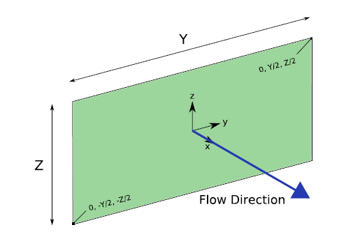
Fig. 1. The geometry of the Domenico solution source plane.

The general form of the Domenico solution used in this model is the three-dimensional transient solution of Martin-Hayden and Robbins (1997), which is based on the work by Domenico and Robbins (1985) and Domenico (1987),

\[ C(x,y,z,t)=\frac{C_0}{8}F_1(x,t)F_2(y,x)F_3(z,x) \]

with

\[ \begin{gathered} F_1 = \exp\left[\frac{x}{2\alpha_x}\left(1-\sqrt{1+\frac{4k\alpha_x}{v}}\right)\right] \times \text{erfc}\left[\frac{x-vt\sqrt{1+\frac{4k\alpha_x}{v}}}{2\sqrt{\alpha_xvt}}\right] \\ + \exp\left[\frac{x}{2\alpha_x}\left(1+\sqrt{1+\frac{4k\alpha_x}{v}}\right)\right] \times \text{erfc}\left[\frac{x+vt\sqrt{1+\frac{4k\alpha_x}{v}}}{2\sqrt{\alpha_xvt}}\right] \end{gathered} \]

\[ F_2=erf\left(\frac{y+Y/2}{2\sqrt{\alpha_yx}}\right)-erf\left(\frac{y-Y/2}{2\sqrt{\alpha_yx}}\right) \]

\[ F_3=erf\left(\frac{z+Z/2}{2\sqrt{\alpha_z x}}\right)-erf\left(\frac{z-Z/2}{2\sqrt{\alpha_z x}}\right) \]

where \(\alpha_x\), \(\alpha_y\), and \(\alpha_z\) are the longitudinal, horizontal transverse and vertical transverse dispersivities \([L]\); \(k\) is the first order decay coefficient \([T^{-1}]\); \(v\) is the groundwater seepage velocity in the longitudinal direction \([LT^{-1}]\), \(Y\) and \(Z\) are the width and height of the source plane respectively \([L]\) and \(t\) is time \([T]\).

The actual form of the Domenico solution used in ArcNLET-Py is the steady-state, two-dimensional version of Equation 3 as follows,

\[ C(x,y)=\frac{C_0}{2}F_1(x)F_2(y,x) \]

\[ F_1=exp\left[\frac{x}{2\alpha_x}\left(1-\sqrt{1+\frac{4k\alpha_x}{v}}\right)\right] \]

\[ F_2=erf\left(\frac{y+Y/2}{2\sqrt{\alpha_y x}}\right)-erf\left(\frac{y-Y/2}{2\sqrt{\alpha_y x}}\right) \]

Equation 7 (along with Equation 8 and 9) is obtained by ignoring vertical dispersion in Equation 3 by setting the transverse vertical dispersivity, \(a_z\), in Equation 6 equal to zero. The error function tends to \(\pm 1\) as the argument tends to \(\pm \infty\). Therefore, when \(-Z/2<z<Z/2\), \(F_3\) becomes \(erf(+\infty)-erf(-\infty)=2\). This makes the solution two-dimensional. To impose a steady-state condition, \(t\) is taken to \(+\infty\). The complementary error function is defined as \(erfc(t)=1-erf(t)\) therefore as the argument tends to \(+\infty\), \(erft(t)\) tends to \(0\) and as it tends to \(-\infty\), it tends to \(2\). Using these properties, as \(t\) goes to \(+\infty\), the term after the addition sign in Equation 4 become \(0\) and the first \(erfc\) term becomes 2. The other terms do not depend on \(t\) and therefore remain unchanged.

2.2 The Relationship between \(M_{in}\) and \(Z\) for a single solute

\(M_{in}\) means the mass input from the source plane, as shown in Figure 1, to groundwater. The calculation of the mass input rate, \(M_{in}\), is more complicated. The input load calculation accounts not only for mass input due to advection from the source plane but also through dispersion of the source plane.

\[ M_{in} = M_{adv}+M_{dsp} \]

The advection term is calculated using the volume of water that flows across the interface (source plane) in unit time, multiplied by the solute concentration,

\[ M_{adv}=C_0YZ\theta v \]

where \(C_0[M/L^3]\) is the concentration of the source plane; \(Y\) and \(Z\) are the dimensions of the source plane \([L]\); \(v[L/T]\) is the seepage velocity, and \(\theta [\text-]\) is the porosity. The dispersion term is calculated by assuming dispersion is governed by Fick’s Law (Freeze and Cherry, 1979). The dispersion through the source plane is written as,

\[ M_{dsp}=-D_{xx}YZ\theta \frac{\partial C}{\partial x} \]

where \(D_{xx} [L^2/T]\) is the component of the dispersion tensor along the x-direction. The dispersion parameters is actually a second order tensor in three dimensions, represented by a \(3 \times 3\) matrix. Because the direction of the principal flow has been aligned with the coordinate system, and the flow is assumed to be only in the \(x\)-direction, all \(y\)-terms, \(z\)-terms and \(x\text{-}y\) cross terms vanish, leaving only the \(D_{xx}\) term.

Disregarding molecular diffusion, the dispersion coefficient is calculated as,

\[ D_{xx} = \alpha_x v \]

where \(\alpha_x [L]\) is the medium’s dispersivity in the \(x\)-direction and \(v[L/T]\) is seepage velocity as before. Putting everything together and \(M_{in}\) can be shown as,

\[ M_{in}=C_0YZ\theta v-\alpha_xYZ\theta v \frac{d C}{d x} \Big|_{x=0} \]

Equation 12 uses the partial derivative symbol \(\partial\) while Equation 14 uses the total derivative symbol \(d\) because x is the only independent variable. The \(\frac{d C}{d x}\) term can be calculated from Equation 7. The remaining terms in Equation 12 are specified parameters or are otherwise known.

Differentiating Equation 7 (using the chain rule) and evaluating it at the location of the source plane,

\[ \frac{d C}{d x} \Big|_{x=0}=\frac{C_0}{2}F_2|_{x=0}\frac{d F_1}{d x}\Big|_{x=0}+\frac{C_0}{2}F_1|_{x=0}\frac{d F_2}{d x}\Big|_{x=0} \]

Calculating \(d F_1/d x\) is straightforward,

\[ \begin{gathered} \left.\frac{d F_1}{d x}\right|_{x=0} &= \frac{d}{d x} \exp\left[ \frac{x}{2\alpha_x} \left(1 - \sqrt{1 + \frac{4k\alpha_x}{v}}\right) \right] \\ &= F_1|_{x=0} \times \frac{1 - \sqrt{1 + \frac{4k\alpha_x}{v}}}{2\alpha_x} \notag \\ &= \frac{1 - \sqrt{1 + \frac{4k\alpha_x}{v}}}{2\alpha_x} \end{gathered} \]

The calculation of \(d F_2/d x\) requires multiple steps. The intermedia variables is used as,

\[ u=\frac{y+Y/2}{2\sqrt{\alpha_yx}}, \quad v=\frac{y-Y/2}{2\sqrt{\alpha_yx}} \]

Therefore,

\[ F_2 = erf(u)-erf(v) \]

The error function is,

\[ erf(z)=\frac{2}{\sqrt{\pi}}\int^{z}_{0}e^{-t^2}dt \]

Based on Leibniz’s integral rule, the derivative of the error function is,

\[ \frac{d}{dz}\left[erf(z)\right]=\frac{d}{dz}\left[\frac{2}{\sqrt{\pi}}\int^{z}_{0}e^{-t^2}dt\right]=\frac{2}{\sqrt{\pi}}\cdot \frac{d}{dz}\left[\int^{z}_{0}e^{-t^2}dt\right]=\frac{2}{\sqrt{\pi}}e^{-z^2} \]

Therefore,

\[ \frac{dF_2}{dx}=\frac{d}{dx}\left[erf(u)-erf(v)\right]=\frac{2}{\sqrt{\pi}}\left[e^{-u^2}\cdot \frac{du}{dx}-e^{-v^2}\cdot \frac{dv}{dx}\right] \]

\[ \begin{gathered} u = \frac{C_u}{\sqrt{x}} \quad \Rightarrow \quad \frac{du}{dx} = -\frac{C_u}{2x^{3/2}} \\ v = \frac{C_v}{\sqrt{x}} \quad \Rightarrow \quad \frac{dv}{dx} = -\frac{C_v}{2x^{3/2}} \end{gathered} \]

\(C_u\) and \(C_v\) are constant parameters, as \(C_u=\frac{y+Y/2}{2\sqrt{\alpha_y}}\), and \(C_v=\frac{y-Y/2}{2\sqrt{\alpha_y}}\).

\[ \begin{gathered} \frac{dF_2}{dx}=\frac{2}{\sqrt{\pi}}\left[e^{-u^2}\cdot \left(-\frac{y+Y/2}{4\sqrt{\alpha_y}\cdot x^{3/2}}\right)-e^{-v^2}\cdot \left(-\frac{y-Y/2}{4\sqrt{\alpha_y}\cdot x^{3/2}}\right)\right] \\ =\frac{1}{2\sqrt{\pi \alpha_y}\cdot x^{3/2}}\left[-\left(y+Y/2\right)e^{-u^2}+\left(y-Y/2\right)e^{-v^2}\right] \\ =\frac{1}{2\sqrt{\pi \alpha_y}\cdot x^{3/2}}\left[-\frac{y+Y/2}{e^{\frac{(y+Y/2)^2}{4\alpha_y x}}}+\frac{y-Y/2}{e^{\frac{(y-Y/2)^2}{4\alpha_y x}}}\right] \end{gathered} \]

The result of this expression depends on the limit value of,

\[ \lim_{x \to 0}\frac{e^{-C/x}}{x^{3/2}} \to 0 \]

where \(C\) is a positive constant value.

As \(x \to 0^+\),

• \(x^{3/2} \to 0^+\), The denominator tends to infinity,

• The numerator \(e^{-C/x} \to 0\), but exponentially fast.

The exponential decay like \(e^{-1/x}\) goes to \(0\) much faster than any power of x goes to infinity, therefore the Equation 24 goes to 0. As a result,

\[ \frac{dF_2}{dx}\Big |_{x=0}=0 \]

Besides,

\[ \begin{gathered} F_2\big|_{x=0}=erf\left(\frac{y+Y/2}{2\sqrt{\alpha_y x}}\right)-erf\left(\frac{y-Y/2}{2\sqrt{\alpha_y x}}\right) \\ =erf(+\infty)-erf(-\infty) =1-(-1)=2 \end{gathered} \]

Then,

\[ \begin{gathered} \frac{\partial C}{\partial x} \Big|_{x=0}=\frac{C_0}{2}F_2|_{x=0}\frac{dF_1}{dx}\Big |_{x=0}+\frac{C_0}{2}F_1|_{x=0}\frac{dF_2}{dx}\Big |_{x=0} \\ =\frac{C_0}{2}F_2|_{x=0}\frac{dF_1}{dx}\Big |_{x=0}+0 \\ =\frac{C_0}{2}\times 2 \times \frac{1-\sqrt{1+\frac{4k\alpha_x}{v}}}{2\alpha_x} \\ =C_0 \cdot \frac{1-\sqrt{1+\frac{4k\alpha_x}{v}}}{2\alpha_x} \end{gathered} \]

Equation 14 can be finally calculated as,

\[ \begin{gathered} M_{in}=C_0YZ\theta v-\alpha_xYZ\theta v \frac{d C}{d x} \Big|_{x=0} \\ =C_0YZ\theta v-\alpha_xYZ\theta v C_0 \cdot \frac{1-\sqrt{1+\frac{4k\alpha_x}{v}}}{2\alpha_x} \\ =C_0YZ\theta v\left(1-\frac{1-\sqrt{1+\frac{4k\alpha_x}{v}}}{2}\right) \\ =C_0YZ\theta v\frac{1+\sqrt{1+\frac{4k\alpha_x}{v}}}{2} \end{gathered} \]

\[ Z=\frac{M_{in}}{C_0Y\theta v}\cdot \frac{2}{1+\sqrt{1+\frac{4k\alpha_x}{v}}} \]

In the solute transport module of ArcNLET-Py, if “Specified Input Mass Rate” is selected, Equation 29 is employed to calculate the \(z\)-value, and the contaminant input mass \(M_{in}\) becomes an essential input parameter. Conversely, if “Specified Z” is chosen, providing the \(z\)-value itself is required as an essential input.

2.3 Considering both ammonium and nitrate

The governing equation used in ArcNLET-Py to calculate both ammonium and nitrate solute transport is the steady-state advection-dispersion equation, which can be presented as,

\[ 0=D_x\frac{\partial^2{C_{NH^{+}_4}}}{dx^2}+D_y\frac{\partial^2{C_{NH^{+}_4}}}{dy^2}-v\frac{\partial{C_{NH^{+}_4}}}{\partial{x}}-k_{nit}\left(1+\frac{\rho k_d}{\theta}\right)C_{NH^{+}_4} \]

\[ 0=D_x\frac{\partial^2{C_{NO^{-}_3}}}{dx^2}+D_y\frac{\partial^2{C_{NO^{-}_3}}}{dy^2}-v\frac{\partial{C_{NO^{-}_3}}}{\partial{x}} \\ +k_{nit}\left(1+\frac{\rho k_d}{\theta}\right)C_{NH^{+}_4}-k_{deni}C_{NO^{-}_3} \]

where the \(D_x\) and \(D_y\) are the dispersivity coefficients in the longitudinal \((x)\) and horizontal transverse \((y)\) directions, respectively; \(c_{NH^+_4}\) and \(c_{NO^-_3}\) are the concentrations of ammonium and nitrate, respectively; \(v\) is groundwater velocity in the longitudinal direction; \(\rho\) is bulk density; \(k_d\) is linear adsorption coefficient of ammonium; \(k_{nit}\) and \(k_{deni}\) are the first-order nitrification and denitrification rates, respectively; and \(\theta\) is porosity.

The boundary conditions for the ammonium and nitrate are as follows,

\[ \begin{gathered} C_{NH_4^+}(0,y)=\begin{cases} C_{0,NH_4^+} &\text{if } -\frac{Y}{2}<y<\frac{Y}{2} \\ 0 &\text{elsewhere} \end{cases} \\ \lim_{x \to \pm \infty}{\frac{\partial C_{NH_4^+}(x, y)}{\partial x}}=0; \lim_{y \to \pm \infty}{\frac{\partial C_{NH_4^+}(x, y)}{\partial y}}=0 \end{gathered} \]

\[ \begin{gathered} C_{NO_3^-}(0,y)=\begin{cases} C_{0,NO_3^-} &\text{if } -\frac{Y}{2}<y<\frac{Y}{2} \\ 0 &\text{elsewhere} \end{cases} \\ \lim_{x \to \pm \infty}{\frac{\partial C_{NO_3^-}(x, y)}{\partial x}}=0; \lim_{y \to \pm \infty}{\frac{\partial C_{NO_3^-}(x, y)}{\partial y}}=0 \end{gathered} \]

Equations 30 and 31 cannot be solved directly using the Domenico solution; instead, a transformation is required. The analytical solutions of Equation 30 and 31 can be obtained by using the method of Sun et al. (1999) that transforms the two coupled equations into two independent equations. This is done by defining the auxiliary variables as,

\[ a_{NH^+_4}=C_{NH^+_4} \]

\[ a_{NO^-_3}=C_{NO^-_3}+\frac{k_{nit}\left(1+\rho k_{d}/\theta\right)}{k_{nit}(1+\rho k_{d}/\theta)-k_{deni}}C_{NH^+_4} \]

With the auxiliary variable, Equations 30 and 31 can be transformed to,

\[ 0=D_x\frac{\partial^2{a_i}}{\partial x^2}+D_y\frac{\partial^2{a_i}}{\partial y^2}-v\frac{\partial{a_i}}{\partial{x}}-k_i a_i \]

\[ \begin{gathered} k_i=\begin{cases} k_{nit}\left(1+\frac{\rho k_d}{\theta}\right) &\text{if } i=NH_4^+ \\ k_{deni} &\text{if } i=NO_3^- \end{cases} \end{gathered} \]

For ammonium, the Domenico solution can be,

\[ C_{NH_4^+}=a_{NH_4^+} \]

\[ a_{NH_4^+}(x,y)=\frac{a_{NH_4^+, 0}}{2}F_{1,NH_4^+}(x)F_{2,NH_4^+}(y,x) \]

\[ F_{1,NH_4^+}=exp\left[\frac{x}{2\alpha_{NH_4^+,x}}\left(1-\sqrt{1+\frac{4k_{nit}(1+\frac{\rho k_d}{\theta})\alpha_{NH_4^+,x}}{v}}\right)\right] \]

\[ F_{2,NH_4^+}=erf\left(\frac{y+Y/2}{2\sqrt{\alpha_{NH_4^+,y} x}}\right)-erf\left(\frac{y-Y/2}{2\sqrt{\alpha_{NH_4^+,y} x}}\right) \]

For nitrate, the Domenico solution can be,

\[ C_{NO_3^-}=a_{NO_3^-}-\frac{k_{nit}(1+\rho k_d/\theta)}{k_{nit}(1+\rho k_d/\theta)-k_{deni}}a_{NH_4^+} \]

\[ a_{NO_3^-}(x,y)=\frac{a_{NO_3^-, 0}}{2}F_{1,NO_3^-}(x)F_{2,NO_3^-}(y,x) \]

\[ F_{1,NO_3^-}=exp\left[\frac{x}{2\alpha_{NO_3^-,x}}\left(1-\sqrt{1+\frac{4k_{deni}\alpha_{NO_3^-,x}}{v}}\right)\right] \]

\[ F_{2,NO_3^-}=erf\left(\frac{y+Y/2}{2\sqrt{\alpha_{NO_3^-,y} x}}\right)-erf\left(\frac{y-Y/2}{2\sqrt{\alpha_{NO_3^-,y} x}}\right) \]

2.4 The Relationship between \(M_{in}\) and \(Z\) for ammonium

For ammonium,

\[ M_{in, NH_4^+} = M_{adv,NH_4^+}+M_{dsp,NH_4^+} \]

\[ M_{adv,NH_4^+}=C_{0, NH_4^+}YZ_{NH_4^+}\theta v \]

\[ \begin{gathered} M_{dsp,NH_4^+}=-D_{xx, NH_4^+}YZ_{NH_4^+}\theta \frac{d C_{NH_4^+}}{d x}\Big|_{x=0} \\ =-\alpha_{x, NH_4^+}vYZ_{NH_4^+}\theta \frac{d C_{NH_4^+}}{d x} \Big|_{x=0} \end{gathered} \]

\[ \begin{gathered} \frac{d C_{NH_4^+}}{d x} \Big|_{x=0}=\frac{C_{0, NH_4^+}}{2}F_{2,NH_4^+}|_{x=0}\frac{d F_{1,NH_4^+}}{d x}\Big|_{x=0}+\\ \frac{C_{0,NH_4^+}}{2}F_{1,NH_4^+}|_{x=0}\frac{d F_{2,NH_4^+}}{d x}\Big|_{x=0} \end{gathered} \]

\[ \begin{gathered} \frac{d F_{1,NH_4^+}}{d x}\Big|_{x=0}=\frac{d}{d x}exp\left[\frac{x}{2\alpha_{x,NH_4^+}}\left(1-\sqrt{1+\frac{4k_{nit}(1+\frac{\rho k_d}{\theta})\alpha_{x,NH_4^+}}{v}}\right)\right] \\ = F_{1,NH_4^+}|_{x=0} \times \frac{1-\sqrt{1+\frac{4k_{nit}(1+\frac{\rho k_d}{\theta})\alpha_{x,NH_4^+}}{v}}}{2\alpha_{x,NH_4^+}} \\ =\frac{1-\sqrt{1+\frac{4k_{nit}\left(1+\frac{\rho k_d}{\theta}\right)\alpha_{x,NH_4^+}}{v}}}{2\alpha_{x,NH_4^+}} \end{gathered} \]

\(F_{1,NH_4^+} = 1\) while \(x=0\).

\(\frac{d F_{2,NH_4^+}}{d x}\Big|_{x=0}\) can be calculated as similar as the processes in Section 2.2, and the result is 0. Therefore,

\[ \begin{gathered} \frac{d C_{NH_4^+}}{d x} \Big|_{x=0}=\frac{C_{0, NH_4^+}}{2}F_{2,NH_4^+}|_{x=0}\frac{d F_{1,NH_4^+}}{d x}\Big|_{x=0}+\\ \frac{C_{0,NH_4^+}}{2}F_{1,NH_4^+}|_{x=0}\frac{d F_{2,NH_4^+}}{d x}\Big|_{x=0} \\ =\frac{C_{0,NH_4^+}}{2}F_{2,NH_4^+}|_{x=0}\frac{dF_{1,NH_4^+}}{dx}\Big |_{x=0}+0 \\ =\frac{C_{0,NH_4^+}}{2}\times 2 \times \frac{1-\sqrt{1+\frac{4k_{nit}(1+\frac{\rho k_d}{\theta})\alpha_{x,NH_4^+}}{v}}}{2\alpha_{x,NH_4^+}} \\ =C_{0,NH_4^+} \cdot \frac{1-\sqrt{1+\frac{4k_{nit}(1+\frac{\rho k_d}{\theta})\alpha_{x,NH_4^+}}{v}}}{2\alpha_{x,NH_4^+}} \end{gathered} \]

\[ \begin{gathered} M_{in,NH_4^+}=C_{0,NH_4^+}YZ_{NH_4^+}\theta v-\alpha_{x,NH_4^+}YZ_{NH_4^+}\theta v \frac{d C_{NH_4^+}}{d x} \Big|_{x=0} \\ =C_{0,NH_4^+}YZ_{NH_4^+}\theta v-\alpha_{x,NH_4^+}YZ_{NH_4^+}\theta v C_{0,NH_4^+} \cdot \frac{1-\sqrt{1+\frac{4k_{nit}(1+\frac{\rho k_d}{\theta})\alpha_{x,NH_4^+}}{v}}}{2\alpha_{x,NH_4^+}} \\ =C_{0,NH_4^+}YZ_{NH_4^+}\theta v\left(1-\frac{1-\sqrt{1+\frac{4k_{nit}(1+\frac{\rho k_d}{\theta})\alpha_{x,NH_4^+}}{v}}}{2}\right) \\ =C_{0,NH_4^+}YZ_{NH_4^+}\theta v\frac{1+\sqrt{1+\frac{4k_{nit}(1+\frac{\rho k_d}{\theta})\alpha_{x,NH_4^+}}{v}}}{2} \end{gathered} \]

\[ Z_{NH_4^+} = \frac{M_{in,NH_4^+}}{C_{0,NH_4^+}Y\theta v}\cdot \frac{2}{1+\sqrt{1+\frac{4k_{nit}(1+\frac{\rho k_d}{\theta})\alpha_{x,NH_4^+}}{v}}} \]

This equation is similar with Equation 29.

2.5 The Relationship between \(M_{in}\) and \(Z\) for nitrate

The following equations use the same derivation method as before, though there are some questionable aspects to consider. First, I will present the derivation approach, and then highlight the problematic points using an example with specific input parameters.

For nitrate,

\[ M_{in, NO_3^-} = M_{adv,NO_3^-}+M_{dsp,NO_3^-} \]

\[ M_{adv,NO_3^-}=C_{0, NO_3^-}YZ_{NO_3^-}\theta v \]

\[ \begin{gathered} M_{dsp,NO_3^-}=-D_{xx, NO_3^-}YZ_{NO_3^-}\theta \frac{\partial C_{NO_3^-}}{\partial x}\Big|_{x=0} \\ =-\alpha_{x, NO_3^-}vYZ_{NO_3^-}\theta \frac{\partial C_{NO_3^-}}{\partial x} \Big|_{x=0} \end{gathered} \]

We can define \(\lambda\) as a variable to simplify the equations:

\[ \lambda = \frac{k_{nit}(1+\rho k_d/\theta)}{k_{nit}(1+\rho k_d/\theta)-k_{deni}} \]

Therefore,

\[ C_{NO_3^-}=a_{NO_3^-}-\lambda a_{NH_4^+} \]

\[ \begin{gathered} \frac{d C_{NO_3^-}}{d x} \Big|_{x=0}=\frac{da_{NO_3^-}}{dx}-\lambda \frac{da_{NH_4^+}}{dx} \\ = \frac{a_{0, NO_3^-}}{2}F_{2,NO_3^-}|_{x=0}\frac{d F_{1,NO_3^-}}{d x}\Big|_{x=0}+ \frac{a_{0,NO_3^-}}{2}F_{1,NO_3^-}|_{x=0}\frac{d F_{2,NO_3^-}}{d x}\Big|_{x=0} \\ -\lambda\left(\frac{C_{0, NH_4^+}}{2}F_{2,NH_4^+}|_{x=0}\frac{d F_{1,NH_4^+}}{d x}\Big|_{x=0}+ \frac{C_{0,NH_4^+}}{2}F_{1,NH_4^+}|_{x=0}\frac{d F_{2,NH_4^+}}{d x}\Big|_{x=0}\right) \end{gathered} \]

\[ \begin{gathered} \frac{d F_{1,NO_3^-}}{d x}\Big|_{x=0}=\frac{d}{d x}exp\left[\frac{x}{2\alpha_{x,NO_3^-}}\left(1-\sqrt{1+\frac{4k_{deni}\alpha_{x,NO_3^-}}{v}}\right)\right] \\ = F_{1,NO_3^-}|_{x=0} \times \frac{1-\sqrt{1+\frac{4k_{deni}\alpha_{x,NO_3^-}}{v}}}{2\alpha_{x,NO_3^-}} \\ =\frac{1-\sqrt{1+\frac{4k_{deni}\alpha_{x,NO_3^-}}{v}}}{2\alpha_{x,NO_3^-}} \end{gathered} \]

As a results,

\[ \begin{gathered} \frac{d C_{NO_3^-}}{d x} \Big|_{x=0}=\frac{da_{NO_3^-}}{dx}-\lambda \frac{da_{NH_4^+}}{dx} \\ =a_{0, NO_3^-}\cdot \frac{1-\sqrt{1+\frac{4k_{deni}\alpha_{x,NO_3^-}}{v}}}{2\alpha_{x,NO_3^-}}-\lambda \cdot C_{0,NH_4^+} \cdot \frac{1-\sqrt{1+\frac{4k_{nit}(1+\frac{\rho k_d}{\theta})\alpha_{x,NH_4^+}}{v}}}{2\alpha_{x,NH_4^+}} \end{gathered} \]

\[ \begin{gathered} M_{in,NO_3^-}=C_{0,NO_3^-}YZ_{NO_3^-}\theta v-\alpha_{x,NO_3^-}YZ_{NO_3^-}\theta v \frac{d C_{NO_3^-}}{d x} \Big|_{x=0}\\ =C_{0,NO_3^-}YZ_{NO_3^-}\theta v -\alpha_{x,NO_3^-}YZ_{NO_3^-}\theta v \cdot \\ \left(a_{0, NO_3^-}\cdot \frac{1-\sqrt{1+\frac{4k_{deni}\alpha_{x,NO_3^-}}{v}}}{2\alpha_{x,NO_3^-}}- \lambda \cdot C_{0,NH_4^+} \cdot \frac{1-\sqrt{1+\frac{4k_{nit}(1+\frac{\rho k_d}{\theta})\alpha_{x,NH_4^+}}{v}}}{2\alpha_{x,NH_4^+}}\right) \end{gathered} \]

\(C_{0,NO_3^-}=a_{0,NO_3^-}-\lambda C_{0,NH_4^+}\), therefore,

\[ \begin{aligned} M_{in,NO_3^-}= & (a_{0,NO_3^-}-\lambda C_{0,NH_4^+})YZ_{NO_3^-}\theta v -\alpha_{x,NO_3^-}YZ_{NO_3^-}\theta v \cdot \\ & \left[\frac{a_{0, NO_3^-}}{2\alpha_{x,NO_3^-}}\cdot \left(1-\sqrt{1+\frac{4k_{deni}\alpha_{x,NO_3^-}}{v}}\right)- \right. \\ & \left. \lambda \cdot \frac{C_{0,NH_4^+}}{2\alpha_{x,NH_4^+}} \cdot \left(1-\sqrt{1+\frac{4k_{nit}(1+\frac{\rho k_d}{\theta})\alpha_{x,NH_4^+}}{v}}\right)\right] \end{aligned} \]

The terms containing \(a_{0, NO_3^+}\) on the right side of this equation combine together, resulting in,

\[ \begin{gathered} a_{0,NO_3^-}YZ_{NO_3^-}\theta v-\alpha_{x,NO_3^-}YZ_{NO_3^-}\theta v \frac{a_{0, NO_3^-}}{2\alpha_{x,NO_3^-}}\cdot \left({1-\sqrt{1+\frac{4k_{deni}\alpha_{x,NO_3^-}}{v}}}\right) \\ =a_{0,NO_3^-}YZ_{NO_3^-}\theta v\left[1-\frac{1}{2}\left({1-\sqrt{1+\frac{4k_{deni}\alpha_{x,NO_3^-}}{v}}}\right)\right] \\ =\frac{a_{0,NO_3^-}YZ_{NO_3^-}\theta v}{2}\left({1+\sqrt{1+\frac{4k_{deni}\alpha_{x,NO_3^-}}{v}}}\right) \end{gathered} \]

The terms containing \(C_{0, NH_4^-}\) on the right side of this equation combine together, resulting in,

\[ \begin{gathered} -\lambda C_{0,NH_4^+}YZ_{NO_3^-}\theta v+\alpha_{x,NO_3^-}YZ_{NO_3^-}\theta v \cdot \lambda \frac{C_{0, NH_4^+}}{2\alpha_{x,NH_4^+}}\cdot \\ \left({1-\sqrt{1+\frac{4k_{nit}(1+\frac{\rho k_d}{\theta})\alpha_{x,NH_4^+}}{v}}}\right) \\ =-\lambda C_{0,NH_4^+}YZ_{NO_3^-}\theta v \cdot \\ \left[1-\frac{\alpha_{x,NO_3^-}}{2\alpha_{x,NH_4^+}}\left(1-\sqrt{1+\frac{4k_{nit}(1+\frac{\rho k_d}{\theta})\alpha_{x,NH_4^+}}{v}}\right)\right] \end{gathered} \]

\(M_{in,NO_3^+}\) is the sum of Equations 64 and 65,

\[ \begin{aligned} M_{in,NO_3^-}= & \frac{a_{0,NO_3^-}YZ_{NO_3^-}\theta v}{2}\left(1+\sqrt{1+\frac{4k_{deni}\alpha_{x,NO_3^-}}{v}}\right)- \\ & \lambda C_{0,NH_4^+}YZ_{NO_3^-}\theta v \cdot \\ & \left[1-\frac{\alpha_{x,NO_3^-}}{2\alpha_{x,NH_4^+}}\left(1-\sqrt{1+\frac{4k_{nit}(1+\frac{\rho k_d}{\theta})\alpha_{x,NH_4^+}}{v}}\right)\right] \\ = & YZ_{NO_3^-}\theta v\ \left\{ \frac{a_{0,NO_3^-}}{2}\left(1+\sqrt{1+\frac{4k_{deni}\alpha_{x,NO_3^-}}{v}}\right) \right. \\ & \left. - \lambda C_{0,NH_4^+}\left[1-\frac{\alpha_{x,NO_3^-}}{2\alpha_{x,NH_4^+}}\left(1-\sqrt{1+\frac{4k_{nit}(1+\frac{\rho k_d}{\theta})\alpha_{x,NH_4^+}}{v}}\right)\right]\right\} \end{aligned} \]

\[ \begin{gathered} Z_{NO_3^-}=\frac{M_{in,NO_3^-}}{Y\theta v} \cdot \frac{1}{\frac{a_{0,NO_3^-}}{2}\cdot m - \lambda C_{0,NH_4^+}\left(1-\frac{\alpha_{x,NO_3^-}}{2\alpha_{x,NH_4^+}} \cdot n \right)} \end{gathered} \]

where

\[ \begin{gathered} m = 1+\sqrt{1+\frac{4k_{deni}\alpha_{x,NO_3^-}}{v}} \\ n = 1-\sqrt{1+\frac{4k_{nit}\left(1+\frac{\rho k_d}{\theta}\right)\alpha_{x,NH_4^+}}{v}} \end{gathered} \]

A significant issue is that \(Z_{NO_3^-}\) can become negative under certain conditions using Equation 67. These problematic cases will be highlighted using an example with specific input parameters.

\[ \begin{gathered} M_{in,NO_3^-}=20000 \, mg \\ Y = 6 \, m \\ \theta = 0.4 \\ v = 0.02 \, m/day \\ C_{0, NO_3^-} = 1 \, mg/L \\ C_{0, NH_4^+} = 50 \, mg/L \\ \alpha_{x, NO_3^-} = 2.113 \, m\\ \alpha_{x, NH_4^+} = 2.113 \, m\\ k_{nit} = 0.0001 \, 1/day \\ k_{deni} = 0.008 \, 1/day \\ \rho = 1.42 \, g/cm^3 \\ k_d = 2 \, cm^3/g \end{gathered} \]

Using these parameters in Equation 67, the calculated \(Z_{NO_3^-}\) value is -383.92.

The following figure presents the results of the centerline ( \(y=0\) ) of NH₄⁺-N and NO₃⁻-N based on Equations 38–45.

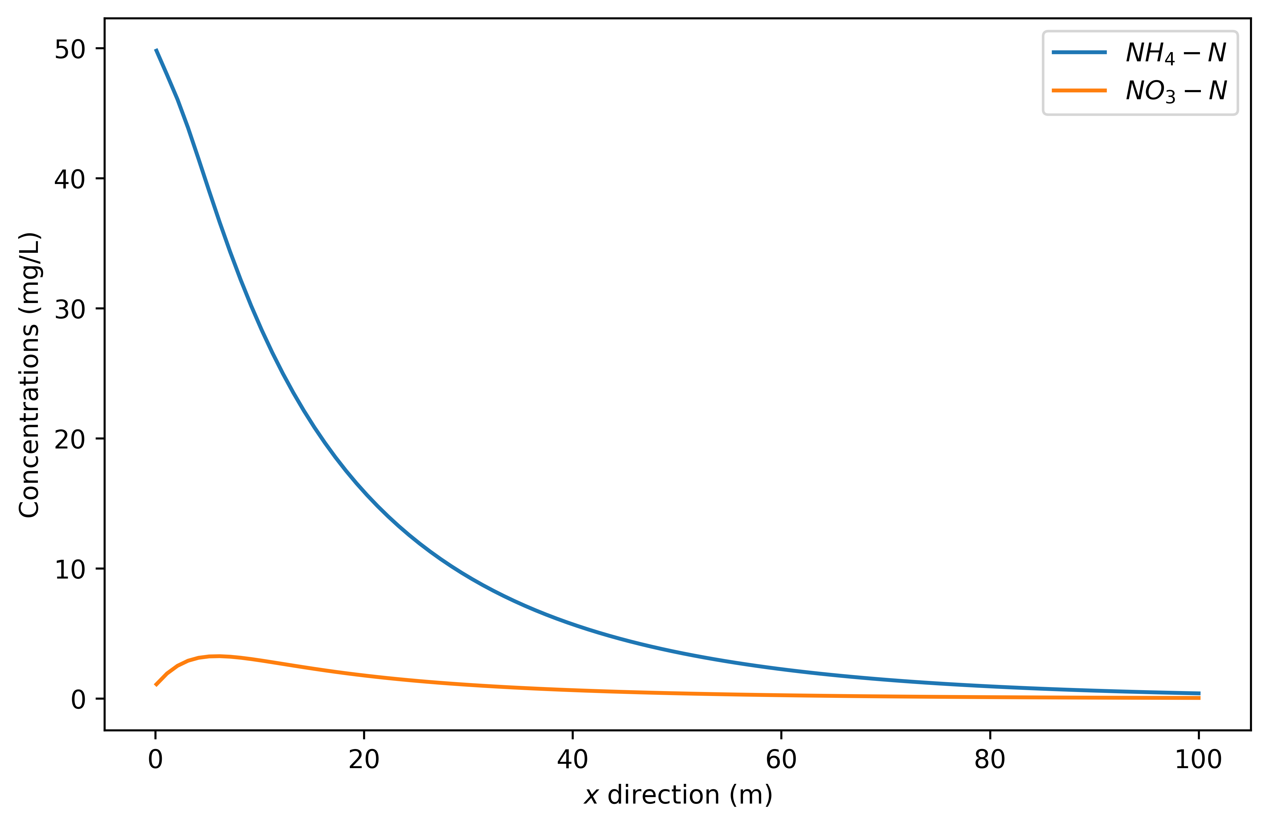
Fig. 2. Centerline ( \(y=0\) ) concentrations of f \(NO_3\text{-}N\) and \(NH_4\text{-}N\), calculated using Equations (38)–(45) with parameters defined in Equation (68). NH₄⁺ and NO₃⁻-N

For NH₄⁺-N, its concentration gradually decreases due to advection, dispersion, and nitrification effects. For NO₃⁻-N, although advection, dispersion, and denitrification processes reduce its concentration, nitrification converts NH₄⁺-N to NO₃⁻-N. When NO₃⁻-N generation through nitrification exceeds the combined reduction effects, the overall NO₃⁻-N concentration increases—this explains the initial rise in NO₃⁻-N shown in Fig. 2.

As shown in Fig. 3, the gray plane represents the nitrate source in groundwater, where nitrate enters the aquifer through both advection and dispersion processes. This leads to the relationship \(M_{in, NO_3^-} = M_{adv,NO_3^-}+M_{dsp,NO_3^-}\) .

In the absence of ammonium, the source plane naturally exhibits the highest nitrate concentration, and dispersion occurs from the source plane along the direction of groundwater flow. In this study, the groundwater flows in the positive \(x\)-direction, which is perpendicular to the source plane. The advective and dispersive contributions of nitrate can be quantified. Their calculation requires both the concentration and the corresponding volume of the nitrate plume. The concentration is obtained using the Domenico solution, while the volume is expressed as a function of \(Z\). This results in a relationship between \(M_{in,NO_3^-}\) and \(Z\), which forms the basis of the previous approach.

However, when both ammonium and nitrate are present, the situation becomes more complex. Nitrate concentrations can increase not only from the source plane but also through nitrification of ammonium. Under certain conditions, the nitrate concentration downstream of the source plane may exceed that within the source plane itself, as shown in Fig. 1. As a result, the dispersion of nitrate may occur in the direction opposite to groundwater flow. If this reverse dispersion is stronger than the advective transport from the source plane, it can result in a negative value for \(M_{in, NO_3^-}\). This explains why, under specific parameter combinations as discussed earlier, our approach may yield a negative value.

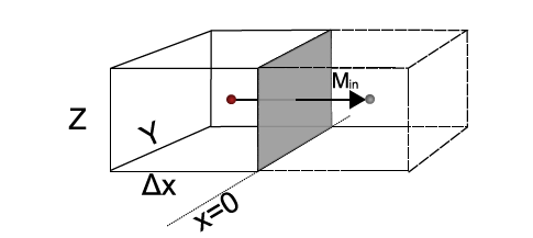
Fig. 3. Mass flux from source plane (gray plane) into groundwater system.

The governing equation of nitrate can be written as,

\[ 0=D_x\frac{\partial^2{C_{NO^{-}_3}}}{dx^2}+D_y\frac{\partial^2{C_{NO^{-}_3}}}{dy^2}-v\frac{\partial{C_{NO^{-}_3}}}{\partial{x}}+k_1-k_2C_{NO^{-}_3} \]

where,

\[ \begin{gathered} k_1=k_{nit}\left(1+\frac{\rho k_d}{\theta}\right)C_{NH_4^+}(x,y) \\ k_2 = k_{deni} \end{gathered} \]

Suppose \(C_{NO_3^-}=C_{1,\,NO_3^-}+C_{2,\,NO_3^-}\), where \(C_{1,\,NO_3^-}\) represents the nitrate from the source plane, and \(C_{2,\,NO_3^-}\) represents the nitrate produced by ammonium nitrification. The first- and second‑order derivative operators are linear and thus satisfy the principle of superposition. Then Equation 70 can be split into,

\[ 0=D_x\frac{\partial^2{C_{1,\,NO^{-}_3}}}{dx^2}+D_y\frac{\partial^2{C_{1,\,NO^{-}_3}}}{dy^2}-v\frac{\partial{C_{1,\,NO^{-}_3}}}{\partial{x}}-k_2C_{1,\,NO^{-}_3} \]

\[ 0=D_x\frac{\partial^2{C_{2,\,NO^{-}_3}}}{dx^2}+D_y\frac{\partial^2{C_{2,\,NO^{-}_3}}}{dy^2}-v\frac{\partial{C_{2,\,NO^{-}_3}}}{\partial{x}}+k_1-k_2C_{2,\,NO^{-}_3} \]

Equation 72 describes the reactive transport of nitrate from the source plane, while Equation 73 describes the reactive transport of nitrate produced by nitrification reactions.

As a results, the \(M_{in,NO_3^-}\) from source plane to groundwater system can be calculated as,

\[ \begin{gathered} M_{in,NO_3^-}=M_{adv,NO_3^-}+M_{dsp,NO_3^-}\\ = C_{0,NO_3^-}YZ_{NO_3^-}\theta v-\alpha_{x, NO_3^-}vYZ_{NO_3^-}\theta \frac{\partial C_{1,\,NO_3^-}}{\partial x} \Big|_{x=0} \end{gathered} \]

Using the Domenico analytical solution for Equation 72 and substituting it into Equation 74, we can obtain the final result:

\[ \begin{gathered} M_{in,NO_3^-}=C_{0,NO_3^-}YZ_{NO_3^-}\theta v-\alpha_{x,NO_3^-}YZ_{NO_3^-}\theta v C_{0,NO_3^-}\cdot \frac{1-\sqrt{1+\frac{4k_{deni}\alpha_{x,NO_3^-}}{v}}}{2\alpha_{x,NO_3^-}} \\ =C_{0,NO_3^-}YZ_{NO_3^-}\theta v \frac{1+\sqrt{1+\frac{4k_{deni}\alpha_{x,NO_3^-}}{v}}}{2} \end{gathered} \]

Therefore,

\[ Z_{NO_3^-}=\frac{M_{in,NO_3^-}}{C_{0,NO_3^-}Y\theta v}\cdot \frac{2}{1+\sqrt{1+\frac{4k_{deni}\alpha_{x,NO_3^-}}{v}}} \]

After deriving numerous formulas and conducting a thorough analysis, we ultimately return to the form of Equation 76.

Figure 4 presents the sensitivity analysis results of \(Z\). Each subplot varies one parameter while keeping others constant at the values from Equation 69. The results demonstrate how different parameter values influence the outcome. For example, at very low velocities, \(Z\) becomes highly sensitive to velocity changes. This sensitivity is expected since \(v\) appears in the denominator of the formula. When \(v\) changes from 10⁻⁵ to 10⁻³ m/day, the seemingly small numerical difference actually represents a significant change of multiple orders of magnitude of \(Z\). Besides, the analysis shows that some parameters, such as \(\rho\), have no effect on \(Z\) values—specifically the \(Z_{NO_3^-}\) calculation. This follows directly from the equations.

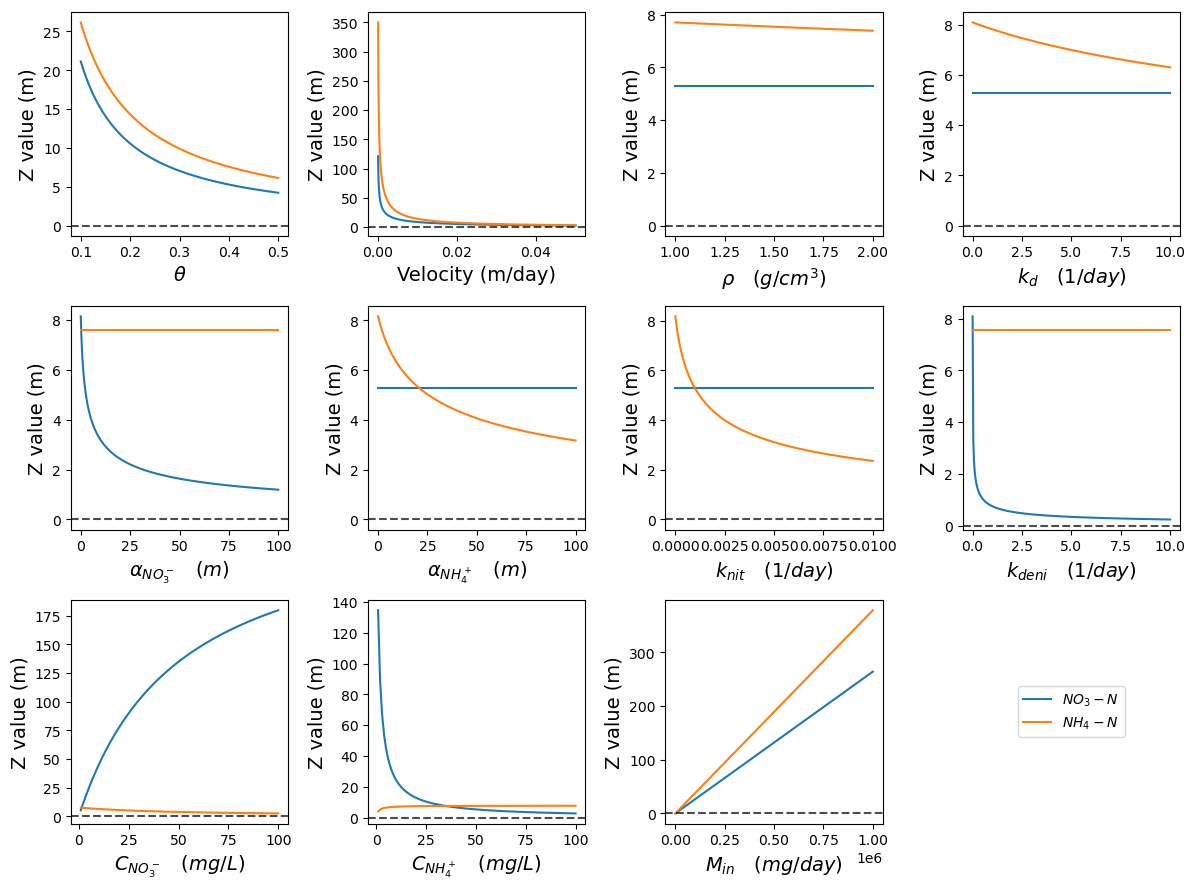
Fig. 4 Sensitivity analysis of \(Z\).

Figure 4 raises another important issue regarding the parameter \(Z_{max}\) in ArcNLET-Py. When calculating \(Z\), the result must not exceed \(Z_{max}\). While the default value of \(Z_{max}\) is 3, the results in Figure 4 demonstrate that calculated \(Z\) values frequently exceed this threshold.

The depths of the plumes were investigated and the results are listed as:

• Turkey Creek study area

The report stated: “the wells were drilled to a depth of 5 feet below the water table or to the top of a sandy clay loam layer encountered at the Groseclose site…” Based on this description of the monitoring well installation, the investigation implicitly assumes that plumes primarily occur within a depth range of 5 feet below the groundwater table, and the groundwater quality monitoring wells were positioned accordingly.

• St. George Island

The report stated: “multi-level samplers (MLS) and 5 cm PVC monitoring wells were installed at all sites to an approximate depth of 3 meters.” Since it is a coastal island with a groundwater table depth of less than 1 m most of the time, the investigation on St. George Island implicitly assumes that the plumes primarily occur within a depth range of 2–3 meters below the groundwater table.

• Wekiva area

For the Seminole County site, the report stated: “based on nitrate concentration contour intervals of 10 mg/L, the \(NO_3\text{-}N\) plume’s maximum dimensions measure approximately 30 feet long by 25 feet wide and approximately 8 feet thick. … Based on total nitrogen concentration contour intervals of 10 mg/L, the plume’s maximum dimensions measure approximately 115 feet long by 75 feet wide and approximately 12 feet thick.”

For the Lake County site, the report stated: “based on nitrate concentration contour intervals of 10 mg/L, the dimensions of nitrate plume … with a total vertical thickness of approximately 14 feet ”

For the Orange County site, the report stated: “based on contour intervals of 10 mg/L, the nitrate plumes dimensions … with a well defined maximum vertical thickness of approximately 12 feet ”

Note that these depths represent the vertical extent where concentrations exceed 10 mg/L. Therefore, the plumes primarily occur within a depth range of 8-14 feet (2.4-4.3 meters) in this site.

• The Soap and Detergent Association Monitoring Site

The groundwater table at the study site is 1.5 to 5 feet below the ground surface. The nitrogen plume reaches its primary depth at 6 feet below the groundwater surface and does not extend significantly beyond 12 feet below ground surface. Based on these measurements, the nitrogen plume roughly has a vertical thickness of 6 feet (2 meters).

• St. Lucie River study area

The M.H.E. PushPoint sampling tool, which is primarily 36 inches in length, was used to sample groundwater. Although the report does not include measured groundwater levels, the use of this shorter length tool implicitly suggests that plumes occur primarily within one foot below the ground surface.

• St. John River Basin (including Eggleston Height, Lakeshore, and Julington Creek)

This study area primarily used PushPoints of 48 and 72 inches in length for groundwater quality monitoring. This implicitly assumes that plumes occur primarily within 4-6 feet below the ground surface.

Based on the monitoring data from multiple study areas, nitrogen plumes are generally confined within a shallow subsurface zone, typically ranging from 1 to 4 meters (3 to 14 feet) below the groundwater table or ground surface. Therefore, setting \(Z_{max}=3\) meters in ArcNLET-Py appears to be a reasonable and representative choice, as it aligns well with the observed vertical extent of nitrogen plumes across diverse field conditions. However, it is important to note that if site-specific measurements of plume depth are available, the “Specified Z” option is recommend and the value of \(Z\) should be adjusted accordingly to reflect actual field observations.

Reference

Domenico, P. A. 1987. An analytical model for multidimensional transport of a decaying contaminant species. Journal of Hydrology 91, 49–58.

Domenico, P. A., Robbins, G. A. 1985. A new method of contaminant plume analysis. Groundwater 23, 4, 476–485.

Martin-Hayden, J. M., Robbins, G. A. 1997. Plume distortion and apparent attenuation due to concentration averaging in monitoring wells. Groundwater 35, 2, 339–346.

Sun, Y., Petersen, J.N., Clement, T.P., Skeen, R.S. 1999. Development of Analytical Solutions for Multispecies Transport with Serial and Parallel Reactions. Water Resources Research 35(1), 185–190.