Preparing Input Data
This section describes several topics for preparing data for ArcNLET-Py. The advanced features of ArcNLET-Py are described via two real-world applications in the Eggleston Heights and Julington Creek neighborhoods in Jacksonville, FL. The underlying model of nitrate fate and transport and the associated algorithmic implementation are described in detail in the technical manual (Rios et al., 2011).
The structure of the manual is as follows: the manual begins with a sensitivity study of the model, which provides the guidelines for model calibration. Then, the procedure for processing LiDAR data to produce a digital elevation model layer (DEM) is discussed. The procedure is followed by two example problems and the model calibration procedure. Finally, the results of nitrate load estimation based on calibrated parameters are shown.
The procedures of preparing a DEM layer based on the National Elevation Dataset (NED), a water body layer based on the National Hydrology Dataset (NHD), and homogenous hydraulic conductivity and porosity layers using raster calculator tool of ArcGIS Pro are fully described in the user’s manual of this software. However, more reliable nitrate load estimation may entail improving the accuracy of NED and NHD data. This manual describes how to achieve this using LiDAR data for its high resolution. On the other hand, for nitrogen load estimation at a relatively large modeling domain, using heterogeneous zones for hydraulic conductivity and porosity parameters is necessary to reflect spatial variability of the site-specific hydrologic conditions. This manual elaborates on how to do so based on soil survey data. For illustration purposes, examples for the Eggleston Heights and Julington Creek neighborhoods in Jacksonville, FL, are used in the discussions below.
Obtaining the Data
Several data sources are available for both the DEM and the water bodies. The sample data for the tutorial was obtained from various sources: the DEM was obtained from the USGS Seamless server, which is not deprecated, while the water body data was obtained from the FDEP (which is based on the National Hydrography Dataset (NHD) data). Both are available at the USGS The National Map (TNM) Download. To illustrate the process of downloading a DEM, the USGS TNM is used as an example. The method outlined describes obtaining a National Elevation Dataset (NED) DEM from the USGS Seamless Server.
Using the National Map Download (TNM) v2 (Figure 7‑1):
Go to TNM Download v2 (nationalmap.gov), and open the Map Viewer.
Zoom to the area of interest.
Select [Map Extent/Geometry] as the Area of Interest.
Under the [Elevation Products (3DEP)] menu, select [1/3 arc-second DEM].
Click the [Search Products] button.
Select the desired area to download by clicking [Download Link (TIF)] (make sure it is large enough to encompass the region of interest).
After selection, a window pops up with the download link.
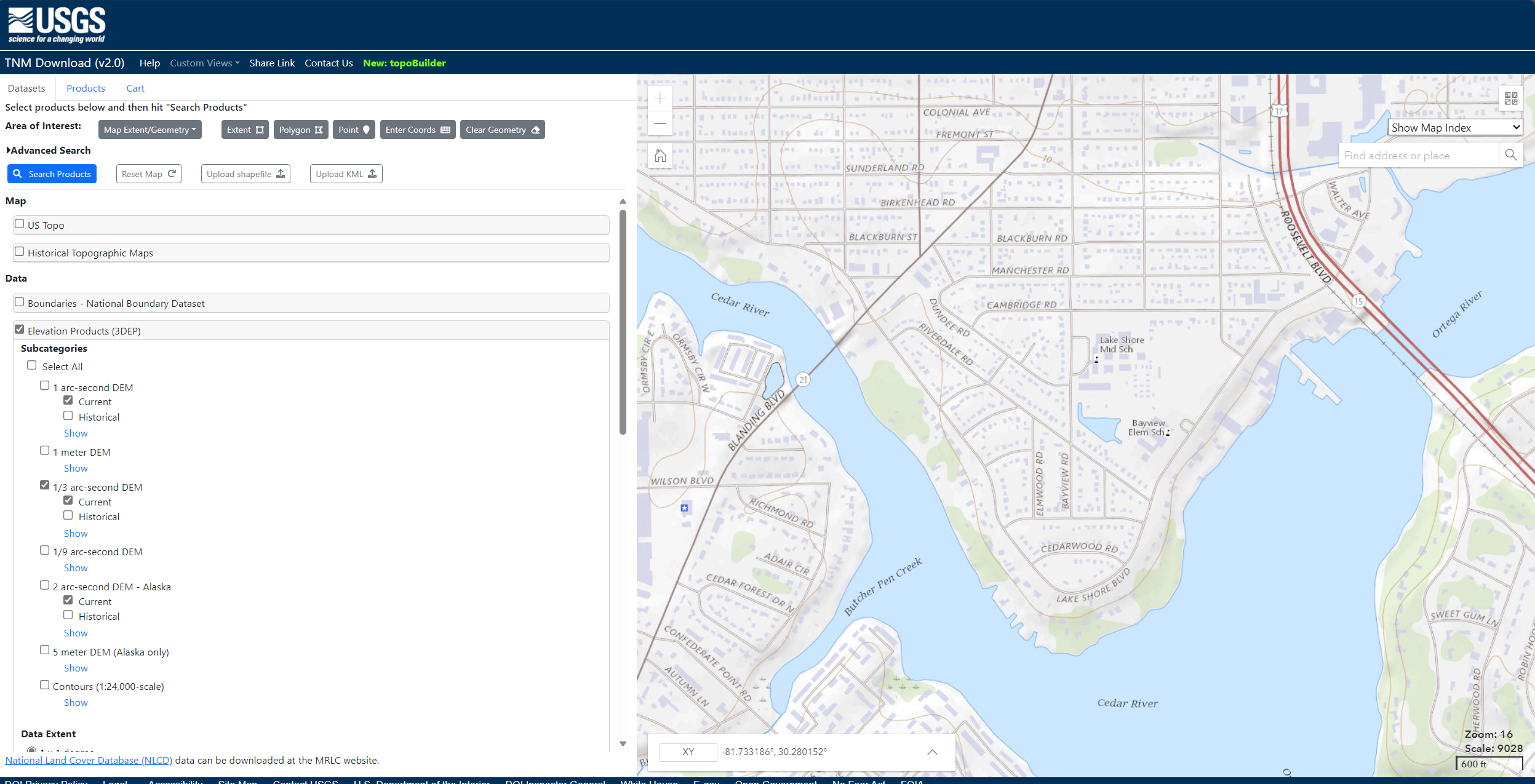
Figure 7‑1: Downloading DEM data using TNM Download.
Although the water body data for this example was obtained from the FDEP, water body data can be obtained from publicly available sources such as the National Hydrography Dataset using the USGS TNM Download TNM Download v2 (nationalmap.gov). (Figure 7‑2)
Go to TNM Download v2 (nationalmap.gov), and open the Map Viewer.
Zoom to the area of interest.
Select [Map Extent/Geometry] as the Area of Interest.
Under the [Hydrography (NHDPlus HR, NHD, WBD)] menu, select [NHDPlus High Resolution (NHDPlus HR)] and [National Hydrography Dataset (NHD)].
Click the [Search Products] button.
Select the desired area to download by clicking [Download Link (ZIP)] (make sure it is large enough to encompass the region of interest). You may need to download more than one file to converge the entire area.
After selection, a window appears with the download link.
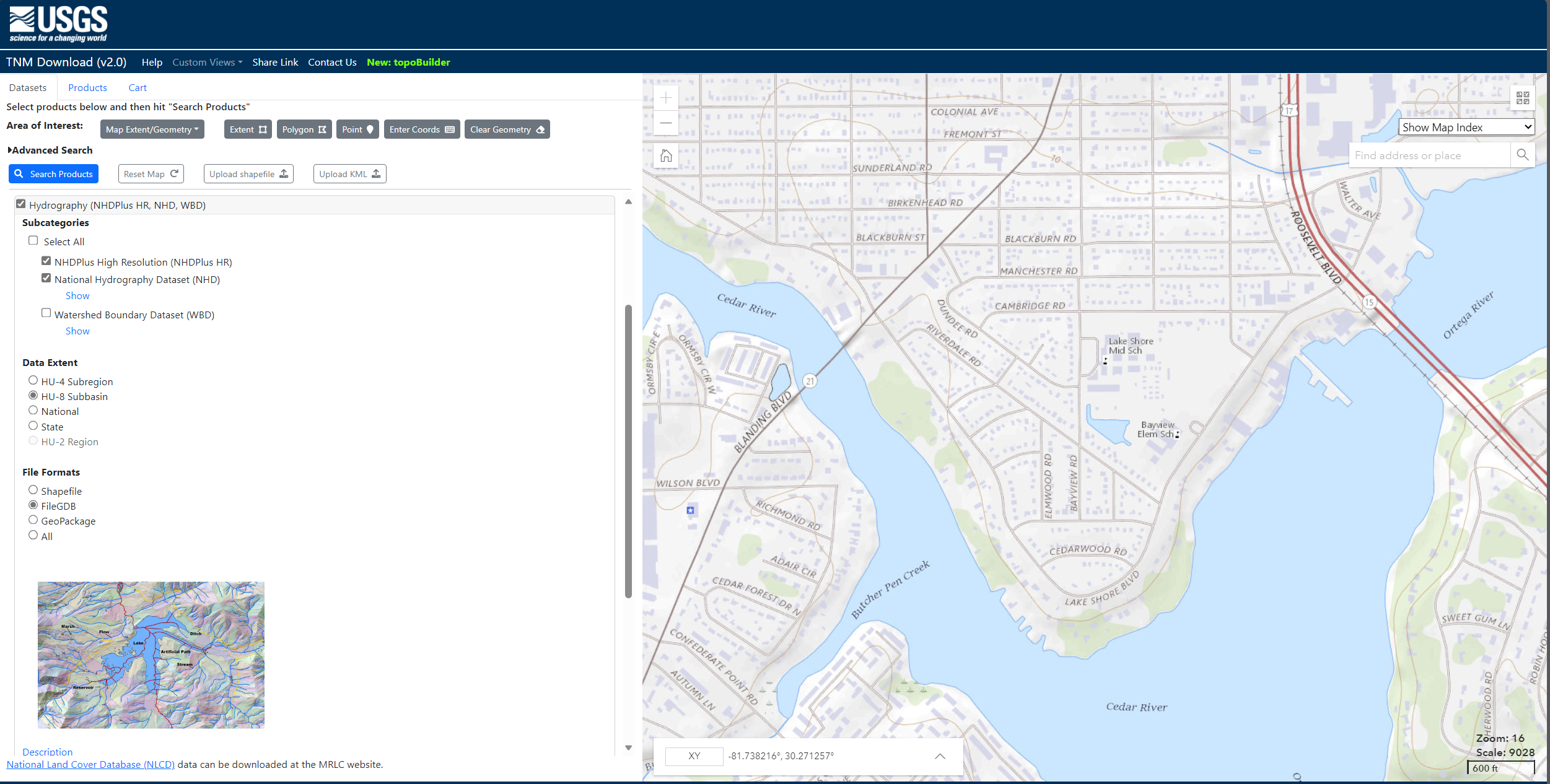
Figure 7‑2: Downloading NHD data.
OSTDS Locations
Another dataset that must be prepared is the source locations. In this example, the source locations (OSTDS) are provided. However, if such a file needs to be created from scratch, a procedure similar to the one used for creating the clipping region is used. The only difference is that instead of creating a polygon feature class, a point feature class is created by making an appropriate selection in the Geometry type dropdown of Figure 7‑8.
Projections
Warning
All model inputs and the map data frame should have the same coordinate system to ensure consistency.
Because the example DEM has elevation units of meters but x- and y-coordinates of degrees, the DEM should be projected into a coordinate system with linear meters units. Projecting the DEM into the correct coordinate system prevents errors in assigning units to model parameters and interpreting the model results. The Universal Transverse Mercator (UTM) is a convenient coordinate system since it is in meter units and uses an easy-to-understand cartesian coordinate system. Since the area of interest lies in UTM Zone 17N, the datasets are projected to this coordinate system. This transformation uses the Project Raster (for the DEM) and Project (for the water bodies) geoprocessing tools of the Data Management toolbox. When projecting the DEM (Figure 7‑3), select Bilinear or Cubic as the resampling technique. For the DEM of this example, change the output cell size from the default value (here, 9.620954m) to 10m, which approximately corresponds to the DEM resolution of 1/3 arc seconds; it is selected for ease of interpretation, and users can select another cell size if desired. As shown in Figure 7‑3, select the output coordinate system NAD_1983_UTM_Zone_17N (this zone encompasses most of Florida). Projecting the water bodies (or any other non-raster format) is straightforward, as the only option required is selecting the output coordinate system, NAD_1983_UTM_Zone_17N, in this example.
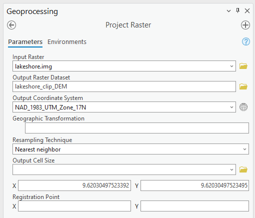
Figure 7‑3: Using the Project Raster tool for clipping the DEM.
The clipped and projected datasets are shown in Figure 7‑4. The final DEM raster should be a floating-point pixel type. The pixel type can be checked by examining the layer properties, as shown in Figure 7‑5. The raster can be converted to a floating-point type using the Float function in the SA toolbox. In addition to checking the data type, the map or data frame’s coordinate system should be set to UTM. If not, this can be done by right-clicking the Map in the Contents Pane and in the Map Properties, selecting NAD 1983 UTM Zone 17N from the list, as shown in Figure 7‑6.
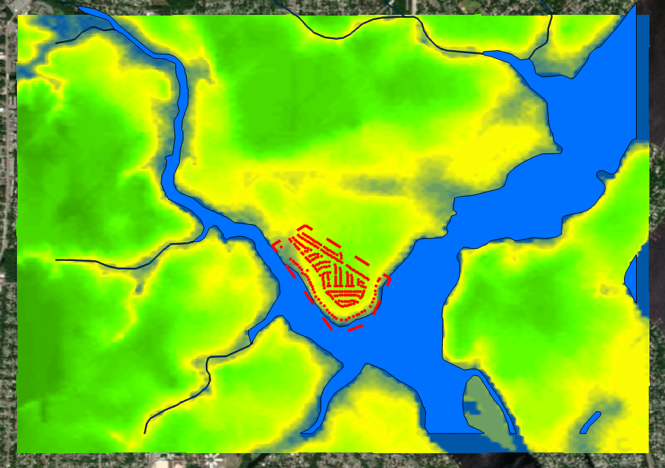
Figure 7‑4: The clipped and projected input data.
The OSTDS are shown as red dots, the study areas (Lakeshore) are shown in a red dashed line, and the DEM ranges from high in green to the water level in blue.
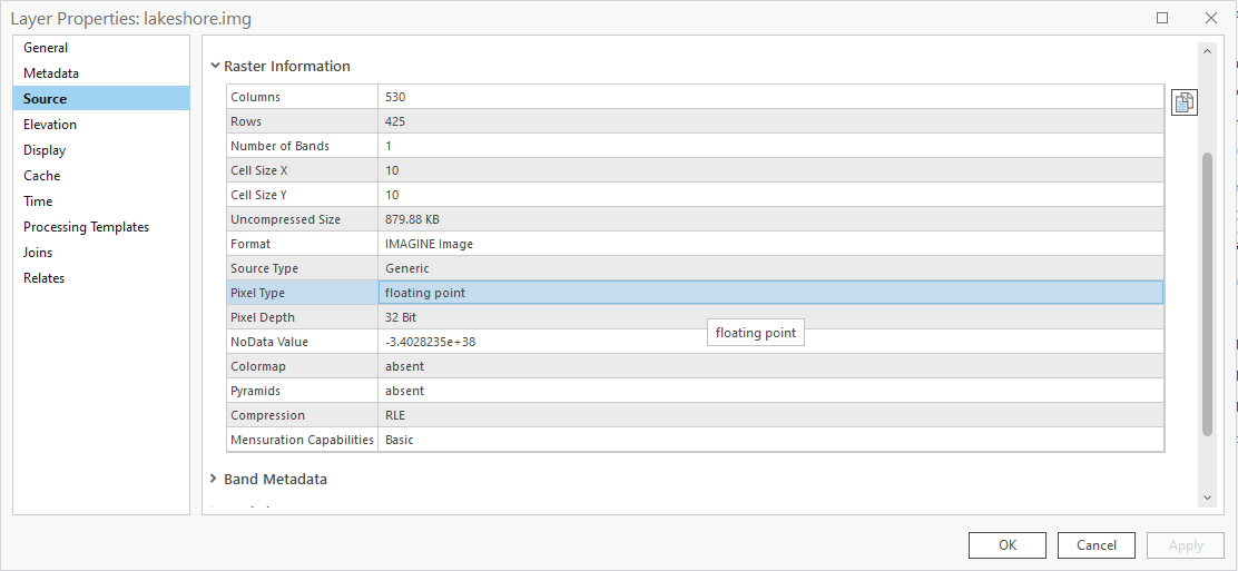
Figure 7‑5: Check for floating point pixel type in layer properties.
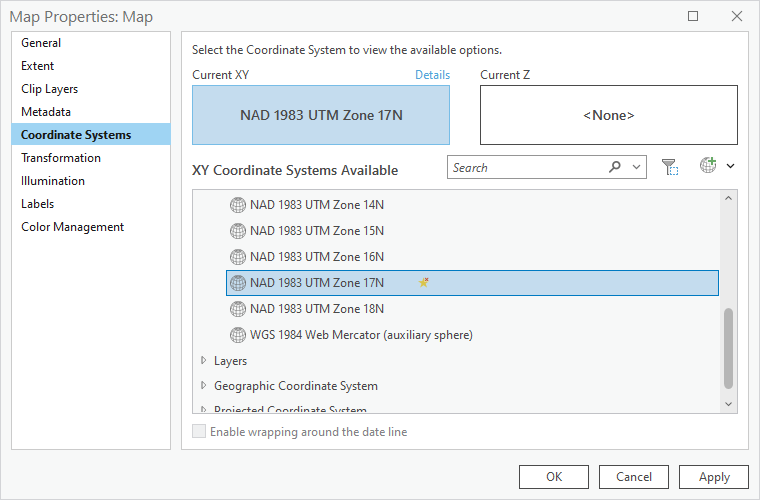
Figure 7‑6: Setting the coordinate system in the map properties.
Clipping
When working with unprocessed data, the first step is to clip all datasets (e.g., DEM, water body, and any other spatial files) to match the extent of the study area. This ensures that the entire study area and all associated files are consistently clipped to the same boundaries. The area of interest in this example is indicated by the dotted outline in Figure 7‑7. It is crucial to clip oversized datasets to the exact extent of the study area to maintain consistency.
A buffer of 0.5 to 1.5 times the dimensions of the study area on all sides should be used. This additional padding ensures that any artifacts caused by calculations near the edges of the domain do not affect the results. By clipping all files to the same study area, consistency across the datasets is maintained, which is essential for accurate modeling and analysis.
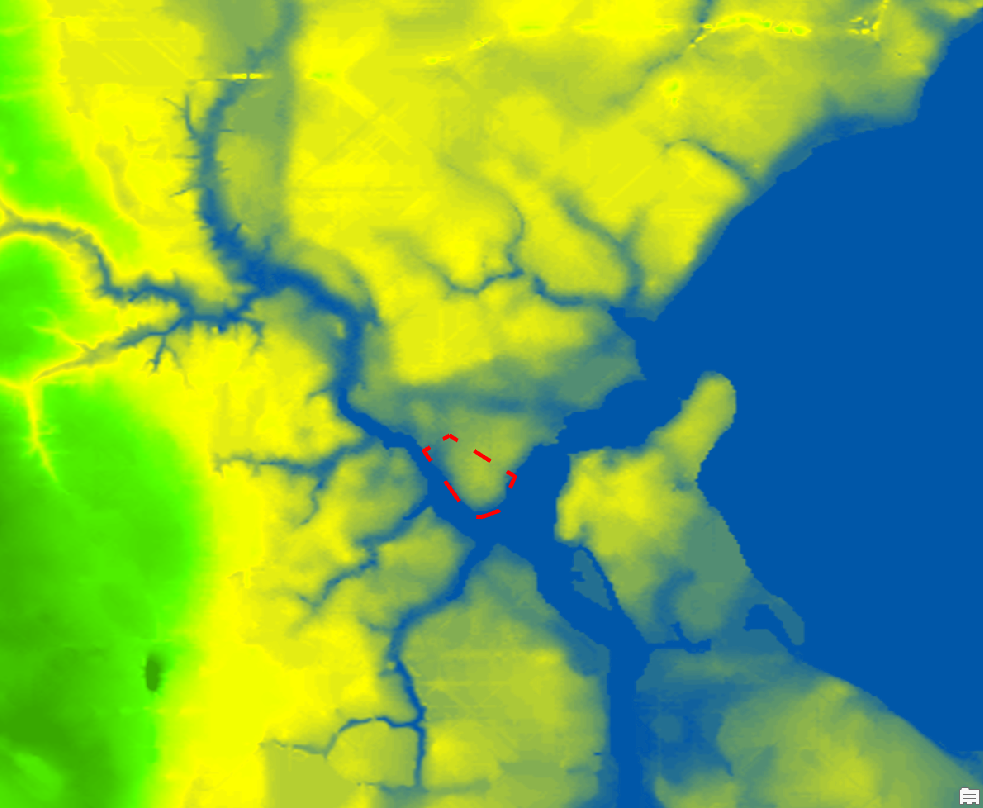
Figure 7‑7: Area of interest within the DEM.
The dashed red lines indicate the Lakeshore neighborhood, and the DEM is the base map that ranges from green and yellow to blue (for the water body).
The clip area can be defined using an existing feature class, or a new clipping region can be created from scratch. To define a new region, create a blank polygon feature class using the Create Feature Class tool in the ArcGIS Pro Geoprocessing Pane, shown in Figure 7‑8. After inputting the feature class location and name parameters, all other options can be left as default.
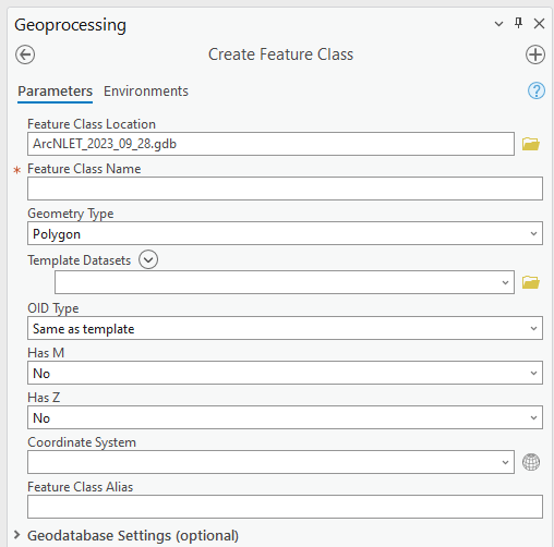
Figure 7‑8: Creating a blank polygon feature class.
After creating the blank feature class, begin with the Edit section on the ribbon in ArcGIS Pro and create a new polygon feature for the desired clipping region using the polygon tool, as shown in Figure 7‑9. Ensure that the editing task is set to Create New Feature and that the target layer is the previously created feature class (Figure 7‑8). After creating the polygon, save the changes via the Edit section of the ribbon (Figure 7‑10).
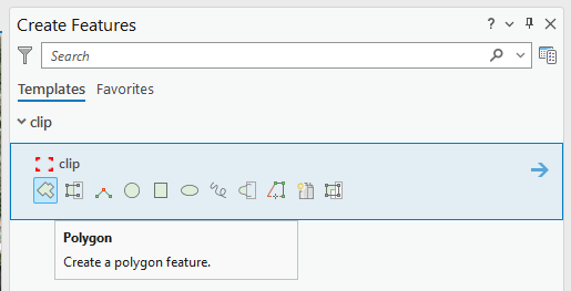
Figure 7‑9: Define a new clipping region.
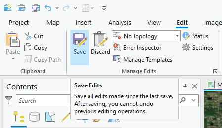
Figure 7‑10: Saving the edits.
After completing the above steps, you should have a clipping region similar to the rectangular region shown in Figure 7‑11.
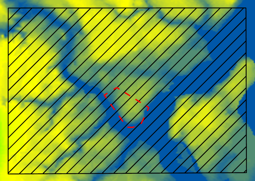
Figure 7‑11: The newly defined clipping region.
The black rectangle with hatch lines denotes the clipping region.
To clip the raster, use the Extract by Mask geoprocessing tool from the SA toolbox shown in Figure 7‑12. Select the DEM as the input raster. Select the newly created clipping region as the mask. Add the extension “.img” to the file name when naming the output raster. Adding the extension uses the ERDAS IMAGINE image format, which is easier to manage and does not have filename length restrictions. Clipping the water bodies (and any other non-raster file, i.e., OSTDS locations) is done with the Pairwise Clip geoprocessing tool from the Analysis toolbox (Figure 7‑13). As the input features, select the water bodies layer. As the clip features, select the clipping region.
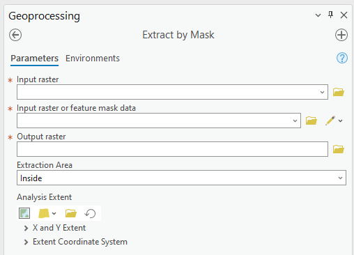
Figure 7‑12: Extract by Mask dialog.
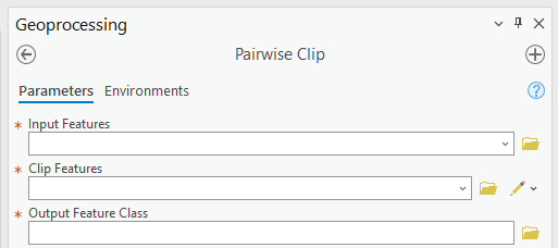
Figure 7‑13: Clipping with features.
Merging Line and Water Bodies Features
Small ditches and streams may be represented as line features in a separate shapefile rather than as polygon features in the main water body shapefile, as with the Lakeshore data. To include these features in the model, they must be incorporated into the main water body shape using the procedure outlined below:
Create a buffer around the line features (NHD_Flowline_DEP_NHD) using the Buffer tool of the Analysis toolbox. The buffer size should be set to a value that appropriately represents the features and is the same or more significant than the DEM cell size. A buffer of 5 meters on each side of the line should be sufficient for this case.
Use the Merge geoprocessing tool of the Data Management toolbox to combine the buffered lines into the water body polygon feature class.
(Optional) Delete any overlapping polygons by removing parts of the buffered flow lines that cover the water body polygons. Find hidden lines by selecting entries from the attribute table and checking if they lay underneath a larger polygon. Merging features reduce the number of water bodies in the shapefile, making it easier to analyze results.
Ensure the final result is in the UTM coordinate system.
Excessive DEM Smoothing
When selecting the amount of smoothing (i.e., determining the value of the smoothing factor in the groundwater module) to perform on a DEM, it should be noted that smoothing by repeated averaging tends to shift the locations of peaks and valleys in the dataset. This is illustrated in Figure 7‑14. The figure’s dotted line represents a hypothetical two-dimensional elevation cross-section of a terrain. The circles mark the locations of the highest and lowest elevation points. The dashed line represents the smoothed elevation profile using various amounts of smoothing. The diamonds mark the locations of the maximum and minimum elevations of the smoothed profile. With one smoothing pass (1x smooth), the locations of the peaks and valleys of the smoothed profile match the unsmoothed profile. As the smoothing amount increases, it is apparent that the locations of the peaks and valleys in the smoothed profile begin to shift, in this case, to the left, which corresponds to the general elevation trend. In the case of 100 smoothing iterations, the peaks have shifted significantly from their original location. If the locations of the valleys coincide with the locations of water bodies (e.g., rivers), the implication is that flow will no longer be towards the water body.
In practice, this effect may produce flow lines that run parallel to the actual location of a river. This phenomenon may sometimes be mistaken for errors in the water body locations or the DEM. If there are errors in the locations of the water bodies, this problem may be exacerbated. This peak/valley shift is a limitation of the smoothing algorithm and is most apparent with small water bodies, i.e., creeks and ponds. It can be mitigated by using smaller smoothing factors (if possible), DEM burning in some instances (see Section 4.7), or by manually shifting the location of the water bodies (if it is determined that doing so would not affect the length of the plumes and the number of plumes intersecting the water body in question).
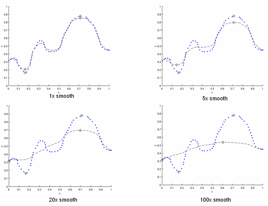
Figure 7‑14: Effect of smoothing on the location of peaks and valleys.
The DEM is a blue line, and the smoothed DEM is in black.
DEM Burning
In certain circumstances, it may be desirable to force groundwater flow towards a water body at a known location, even though flow may not naturally be towards it, as a result. An approach that can be used to force flow toward the desired water bodies is a technique known as DEM burning. The simplest form consists of creating a deep valley or pit in the location of the water body. After calculating flow directions, the flow towards this artificially created pit or valley. This simple DEM burning can be accomplished with the ArcGIS Raster Calculator tool. For example, the following command can be used to create a valley that is 30 units deep in the location of all the water bodies on the map.
Where [water bodies] is the raster representation of the water bodies layer, and [DEM] is the DEM to burn. Note that DEM burning does not produce the desired result in all cases (e.g., it may not work in cases where excessive smoothing has caused a shift in the location of peaks and valleys in the DEM) and may introduce unnatural-looking flow paths. It is left to the modeler’s discretion whether or not to perform DEM burning.
Multiple Smoothings
Suppose small water bodies such as ditches and canals are not reflected in the hydraulic gradient produced in the Groundwater Flow Module and do not impact the particle flow paths as expected. In that case, the solution is to build the small water bodies into the smoothed DEM (the optional output of the Groundwater Flow Module) so that the small water bodies can control the shape of the approximated water table and groundwater flow paths. The phenomena are related to the impacted surface-water drainage network effects on the groundwater gradient, and resultant flow path lines are not fully recognized in the model due to over-sampling (creating a raster that is too coarse) when projecting the LiDAR DEM and the smoothing operation in the Groundwater Flow Module.
This issue is exemplified by groundwater from certain OSTDS not flowing into the nearby ditches. The missing small water bodies relate to the conceptual model of groundwater flow based on which ArcNLET modules of groundwater flow and particle tracking are developed. In the current conceptual model, the small water bodies do not control local groundwater flow because the relation between the ditches and groundwater flow is mainly unknown. In other words, groundwater is controlled by the hydraulic head of the neighborhood scale, whose shape is approximated by the Groundwater Flow Module and can be seen in the optional smoothed DEM output that ArcNLET generates.
Figure 7‑15 illustrates groundwater flow in the current groundwater conceptual model in which the ditches do not control local groundwater flow. The blue lines in Figure 7‑15 represent flow paths from septic tanks (red square) estimated by ArcNLET using a smoothing factor of 60. Three profiles of DEM along the black line marked in Figure 7‑15 are plotted; the black line intersects two ditches. Examining the three profiles shows that:
The profile at the left, titled Original LiDAR DEM (5 x 5 ft2), is based on the original LiDAR DEM with 5 × 5 ft2 resolution (provided by FDEP), and the two ditches are revealed as the two deep valleys on the profile. It suggests that the LiDAR DEM can reflect ditches, including intermittent ones, at the local scale. The LiDAR DEM is projected to the NAD 1983 UTM Zone 17N coordinate system, and the elevation unit is converted from foot to meter.
The profile in the middle, titled Resampled LiDAR DEM (10 x 10 m2), is for the resampled (projected) DEM, from 5 × 5 ft2 to 10 × 10 m2 resolution. (Note that using a raster cell size of 3 x 3 m2 is recommended for ArcNLET.) The resampling is to save computational time for ArcNLET modeling. The profile of the smoothed DEM shows that the resampling resolution is too coarse for the two narrow ditches in that the two ditches are not retained. This problem illustrates the tradeoff between finer resolution and reasonable computational time determined by users to meet their specific project needs. The solution to this problem is to increase the resampling resolution; in the discussion below, the resolution is empirically increased from 10 × 10 m2 to 5 × 5 m2.
The profile at the right, Smoothed DEM (SmthFactor=60), is the smoothed DEM obtained after 60 times of smoothing of the resampled DEM. While large-scale spatial variability is preserved, local-scale variability disappears after the smoothing. As a result, for OSTDS down-gradient of (right to) the peak shown in the profile, groundwater from them flows in the down-gradient direction, i.e., to the right. This explains why groundwater from certain OSTDS does not flow into nearby ditches. As shown below, smoothing is the dominant reason for the disappearing ditches, even when ditches are retained in the resampled DEM.
The above observations are the basis for the proposed solution below to meet the expectation that localized groundwater-table depression occurs near wet ditches. Note that the smoothed DEM is not a default output raster file of ArcNLET. To produce it, one needs to enter the name of the output raster in the [(Optional) Output Smoothed DEM] field in the Groundwater Flow Module to determine the impact on wet ditches. Making multiple smoothed DEMs using various [Smoothing Factor] values may be helpful, too. Including the smoothing factor value in the output, names are valuable for record keeping and determining the best solution.
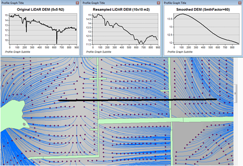
Figure 7‑15: Simulated flow paths from OSTDS with smoothing.
The OSTDS (red squares) are the origins of the paths (blue lines), and the paths are generated by running ArcNLET with a smoothing factor of 60. The three profiles along the black line marked in the figure are the original LiDAR DEM of 5 × 5 ft2 resolution (left), the resampled LiDAR DEM of 10 × 10 m2 resolution (middle), and the smoothed DEM (right) based on the resampled LiDAR DEM. The flow paths are estimated based on the smoothed DEM.
The instructions below detail a solution to build the ditches into the smoothed DEM so that the ditches control the shape of the approximated water table and, subsequently, groundwater flow paths. The instructions are as follows:
When resampling the [LiDAR DEM] (Figure 7‑15 (left)), determine the appropriate resolution so that local ditches are retained in the [resampled DEM].
Although this step may be automated, it remains empirical at this stage. The results are presented below for the resolution of 5 × 5 m2.
Extract the elevations of water bodies, including the ditches, from the [resampled DEM] (Figure 7‑15(middle)). Extract by Mask in the SA Toolbox in ArcGIS can extract the elevation values using water body data (raster or polygon).
The extracted elevations are merged into the [smoothed DEM] in a later step so that the ditches can control groundwater flow paths calculated from the [smoothed DED].
Conduct smoothing by running the Groundwater Flow Module. As shown below, the ditches may disappear after smoothing, although they are retained in the [resampled DEM]. Since the [smoothed DEM] is needed for the next step, we need to type a file name into the [(Optional) Output Soothed DEM] filed to save the DEM.
Including the [Smoothing Factor] value in the output file name is good practice.
Add the extracted elevation of water bodies obtained from the [resampled DEM] to the [smoothed DEM]. Merging these datasets can be done using the Mosaic function in the Data Management Toolbox in ArcGIS.
This step warrants that the [smoothed DEM] at ditches is lower than that of nearby OSTDS.
b. Since the ditch elevations were not used to calculate the hydraulic gradient, the hydraulic gradient is still the same as that of [smoothed DEM] output in the above step. In other words, the ditches still do not control groundwater flow paths toward the ditches for some OSTDS.
To use the elevation of the ditches added to the [smoothed DEM], conduct another round of smoothing in the Groundwater Flow Module so that the ditches added in the step above are used to calculate the hydraulic gradient near the ditches.
The [Smoothing Factor] value should be small, i.e., 2, because a large value for the [Smoothing Factor] may, once again, eliminate the ditches.
This step changes the hydraulic gradient near the ditches.
Run the Particle Tracking Module to simulate the flow paths. If the flow paths are unsatisfactory, repeat Steps 4 and 5 until the expectation is met. Repeating the process results in the ditches having more control of groundwater flow paths.
If hydraulic head measurements are available, then use them as the criteria to determine when to stop the iterative process.
While this procedure is empirical, it may be automated if the procedure is accepted. For example, the water body elevation can automatically be added to the [smoothed DEM] before each smoothing iteration.
The results of the above operations are seen in Figure 7‑16, which plots the simulated groundwater flow path and several profiles. The results are for the 5 × 5 m2 resolution in the resampled DEM. Each profile is discussed below:
The profile at the left of row 1, titled Original LiDAR DEM (5 x 5 ft2), is based on the original LiDAR DEM with 5 × 5 ft2 resolution provided by the FDEP. It is the same as the profile shown in Figure 7‑16 (left).
The profile in the middle of row 1, titled Resampled LiDAR DEM (5 x 5 m2), is based on the resampled DEM produced in Step 1 above by resampling the LiDAR DEM to 5 × 5 m2 resolution. The profile shows that the two ditches are retained with this resolution, while small-scale variability disappears after the resampling.
The profile at the right of row 1, titled Smoothed DEM (Smoothing Factor=60), is the smoothed DEM generated by the Groundwater Flow Module using a smoothing factor of 60, which is the result of Step 3. It shows that the two ditches disappear due to the smoothing, although they were retained in Step 1.
The profile at the left of row 2, title Smoothed DEM (60) + Water Bodies (WB), is the DEM after adding the extracted elevations of water bodies to the smoothed DEM. The extracted elevation file is represented with a WB in the plots in Figure 7‑16 and was obtained in Step 2. The use of the Mosaic function of ArcGIS is the result of Step 4. The profile shows the two ditches. Since the ditches have not been used to calculate the hydraulic gradient, the gradient is the same as that of smoothed DEM in Step 3. As a result, for the left ditch in the plots, the groundwater flow paths travel from the OSTDS in a rightward direction and, in some cases, away from the adjacent ditch. After the hydraulic gradient is adjusted for using the ditch data, groundwater flow paths are impacted by the proximal ditch and flow rightward and leftward towards the ditch.
The profile in the middle of row 2, titled Smoothed DEM (60) + WB (2), is the DEM after smoothing the DEM twice using a smoothing factor of 2 in the Groundwater Flow Module. This profile shows that the hydraulic gradient near the ditches changes after the ditches’ elevation is used for smoothing. Retake the left ditch as an example. Before the smoothing, the hydraulic gradient is only in a rightward direction, both away and towards the ditch. After the smoothing, the gradient near the ditch becomes leftward and rightward towards the ditch, implying that groundwater flows into the ditch for the adjacent OSTDS.
The profile at the right of row 2, titled Smoothed DEM (60) + WB (2) + WB, is based on the raster Smoothed DEM (60) + WB (2) from the plot in the middle of row 2. The results are obtained by adding the water body elevations back to said raster from the step above.
The profile in row 3, titled Smoothed DEM + WB (2) + WB (2), is based on smoothing the raster file for the plot Smoothed DEM (60) + WB (2) + WB twice using the Groundwater Flow Module. Since this profile is similar to that in the middle of row 2, titled Smoothed DEM (60) + WB (2), the decision is to use the flow velocity corresponding to the raster for the plot Smoothed DEM (60) + WB (2) + WB (2) for flow path calculations.
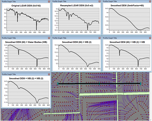
Figure 7‑16: Simulated flow paths from OSTDS with ditches.
The paths are (blue lines) from OSTDS (red squares). The paths are generated by running ArcNLET with a smoothing factor of 60.
The seven profiles along the black line marked in Figure 7‑16 are the original LiDAR DEM of 5 × 5 ft2 resolution (left of row 1), the resampled LiDAR DEM of 5 × 5 m2 resolution (middle of row 1), the smoothed DEM (right of row 1) based on the resampled LiDAR DEM, the smoothed DEM with ditch elevation added (left of row 2), the smooth DEM after two times of smoothing (middle of row 2), the smoothed DEM after two times of smoothing with ditch elevation added (right of row 2), and the smoothed DEM with another two times of smoothing (row 3). The flow paths are estimated based on the smoothed DEM corresponding to the profile of row 3.
In ArcNLET-Py, the model can extract the elevations of water bodies and merge them into smoothed DEM automatically. The user just needs to turn on the “Merge Water bodies” option, and fill in the appropriate number of times to smooth after merging.
Processing LiDAR data
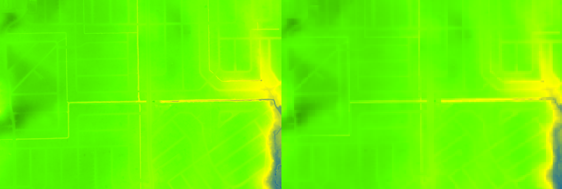
LiDAR DEM is used in both the Eggleston Heights and Julington Creek neighborhoods. The necessity of using LiDAR DEM instead of NED DEM data is demonstrated in the Eggleston Heights neighborhood. Many ditches and canals are in this area (Figure 7‑17, top), but many are narrower than 10m (the 1/3 arc second resolution of the NED DEM used in the user’s manual). As a result, such ditches and canals (i.e., those highlighted in Figure 7‑17, top) cannot be reflected in the NED DEM data (Figure 7‑17, bottom).
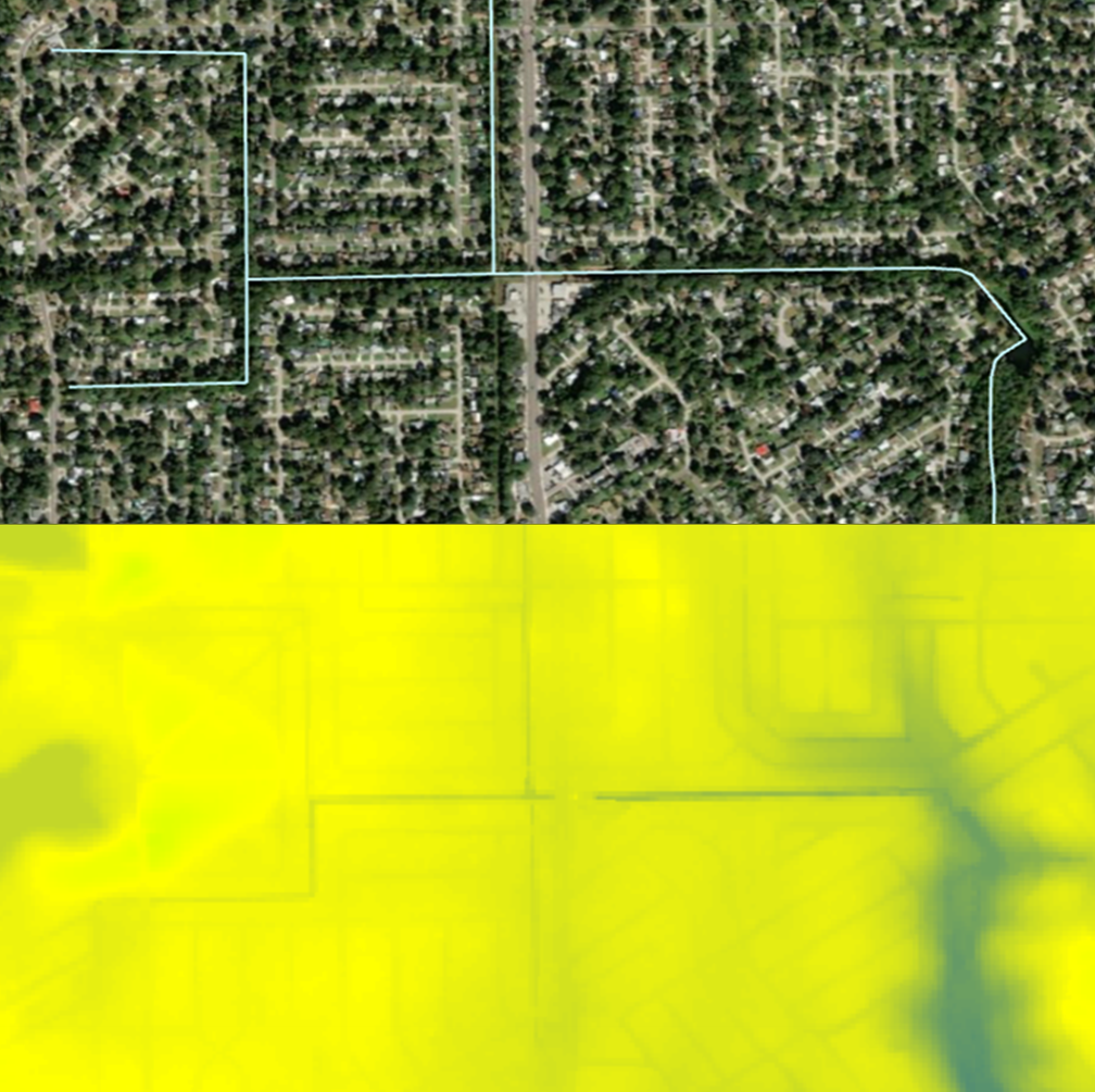
Figure 7‑17: Ditch coverage and 1/3 arc-second DEM (bottom).
The ditch coverage (top) is highlighted in blue and cannot be fully reflected in the 10-m DEM data (bottom).
The LiDAR data with a horizontal resolution of 1 × 1 m2, as shown in Figure 7‑18 left, can represent the ditches, taking in the red ellipse in Figure 7‑17 and Figure 7‑18. As explained in the technical manual (Rios et al., 2011), DEM data of finer resolution always has a highly intense elevation fluctuation and is inconsistent with the water table. On the other hand, it takes longer computation time to smooth DEM data of higher resolution (see the details of smoothing in the technical manual of Rios et al., 2011). Therefore, the LiDAR DEM needs to be processed to reduce the resolution. This study’s targeted resolution is 10 × 10 m2, consistent with the example data associated with the user’s manual. The processed LiDAR DEM is shown in Figure 7‑18 (right), where the ditch in the red ellipse is preserved. The ditches and canals can be better preserved if the target resolution of the processing DEM is smaller than the water features. However, as explained before, a finer resolution may result in a longer computation time of smoothing. Users determine the tradeoff between finer resolution and reasonable computation time to meet their project needs.
7‑18: LiDAR data before and after projecting. Figure
The DEM before projecting (left) and using projecting to change resolution from 1 × 1 m2 to 10 × 10 m2 (right). The ditch highlighted in yellow is better preserved after the projection.
Changing the resolution from 1 × 1 m2 to 10 × 10 m2 is done using the Projections and Transformations → Data Management Tools → project raster tool. As shown in Figure 7‑19 Figure 2-3, when using this tool, the cell size is changed to 10, and the nearest neighbor assignment resampling technique is used. The same tool is used for projection in Section 4.3.
The DEM resolution of 10m discussed above is only for demonstration. Our empirical experience is that the resolution of 10m is always too coarse, and the resolution of 3m is better for providing more reasonable flow paths. The DEM with a 3m resolution is always available on the USGS TNM website. Using a LiDAR DEM does not warrant good results of flow paths because the water table is only a subdued replica of topography. A user may examine the results of the groundwater path based on different DEM resolutions to select the resolution appropriate to their project needs.
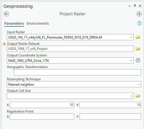
Figure 7‑19: Projecting the LiDAR data.
The geoprocessing tool shows the options to change the raster cell size to a coarser resolution of 10 × 10 m2 (output cell size).
LiDAR DEM Updating Water Bodies
Generally speaking, the accuracy of the water body layer downloaded from the USGS National Hydrography Dataset (NHD) can meet the requirements of ArcNLET-Py, and the NHD data can be used directly in ArcNLET-Py. However, in some areas, NHD data errors regarding water body locations may cause an inaccurate flow path generated by the Particle Tracking Module of ArcNLET. In this case, we suggest updating the NHD data using the LiDAR DEM because LiDAR DEM can reflect water body locations. An example is shown in Figure 7‑20. In the left figure, the LiDAR DEM shows a lower elevation area within the red circle, which appears to be a ditch or canal in the aerial imagery map at the right of Figure 7‑20. However, this water body does not exist in the NHD map. Instead, only a segment of the misplaced flow line (the blue line in the figure) exists in this area. Because of the mismatch between the LiDAR DEM and the NHD data, as shown in the left figure, the simulated flow paths of ArcNLET cannot reach the water body shown as a flow line in Figure 7‑20. The trapped flow paths are physically unreasonable and may cause nitrate load estimation errors. Therefore, the NHD data needs to be updated so that the location and shape of the water body can be accurately represented. In this manual, the update is conducted manually using the LiDAR DEM. The DEM is updated by first generating an evaluation contour map based on the LiDAR DEM using the Spatial Analyst Tools→ Surface → Contour tool, as shown in Figure 7‑21. Based on the generated contour, one can update the water body map using the Editor tool of ArcGIS. The water bodies map before and after the updating are shown in Figure 7‑22. After updating, the simulated flow paths of ArcNLET-Py are smoother and more physically reasonable (Figure 7‑23).
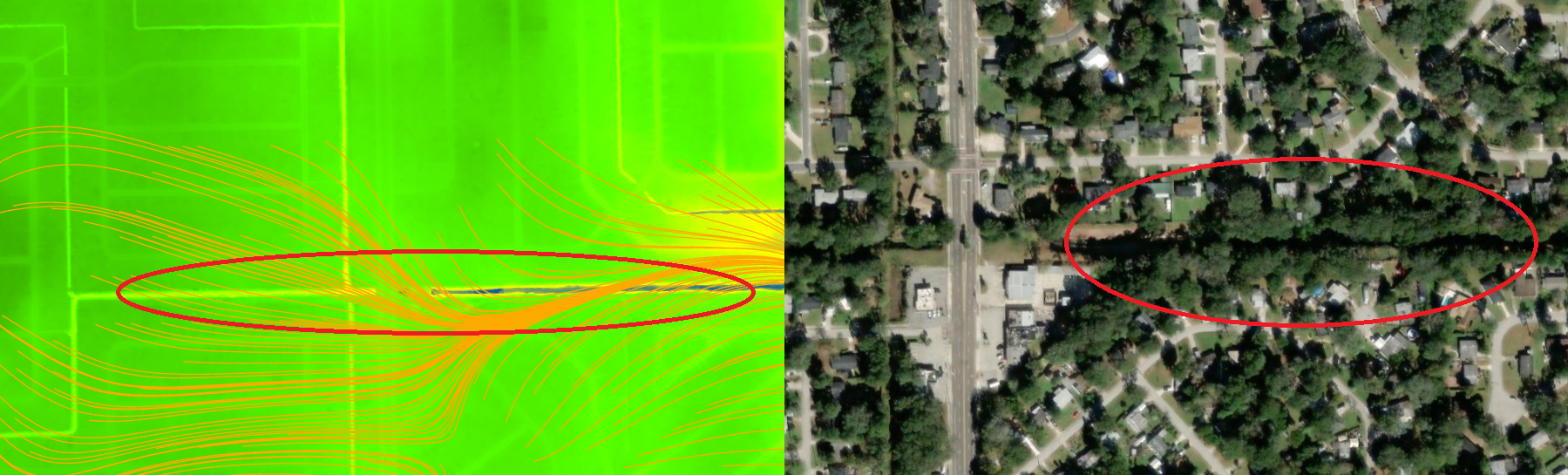
Figure 7‑20: LiDAR DEM and NHD missing features.
The simulated particle path and Esri aerial imagery are shown in the Eggleston Heights neighborhood, Jacksonville, FL. The path is the flow path calculated by the Particle Tracking Module, and the LiDAR DEM is 1 × 1-meter resolution.
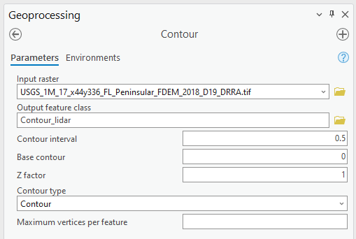
Figure 7‑21: Generating elevation contour based on LiDAR DEM.
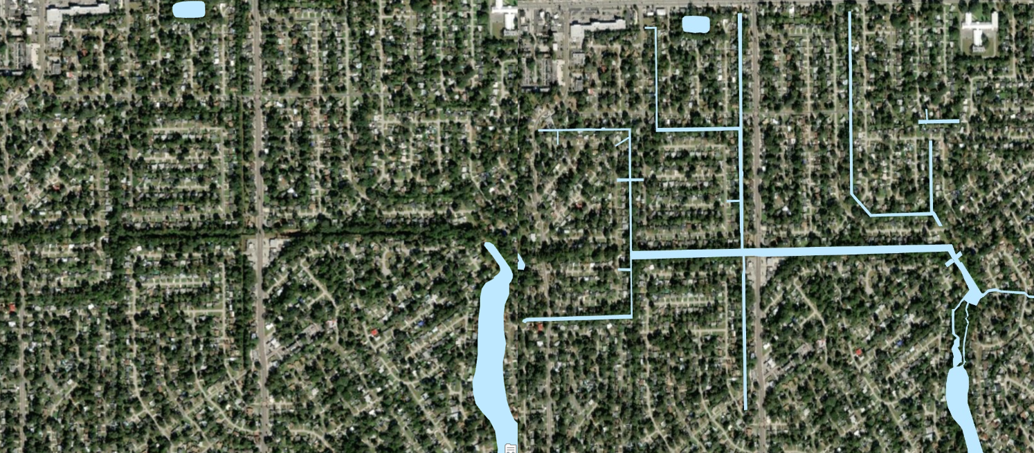
Figure 7‑22: Updating the water body features.
The changes to the water body, shown in blue, can be seen via the before aerial (left) and after aerial (right) updating.
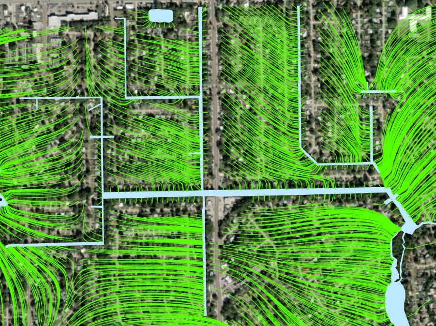
Figure 7‑23: The simulated flow paths after updating the water bodies.
The updated water body features are in blue, and the green particle paths are flowing into the surface waterbodies that were added to the study area.
Units
To ensure consistency and ease of use, the ArcNLET model is fixed to use meters per day as the standard unit of measurement.
This decision was made to avoid potential errors that could arise from users employing different units without recalibrating default parameters.
ArcNLET provides default values for various parameters to simplify the modeling process:
In the transport module, the nitrate dispersivity values are set to: - αL = 2.113 meters per day - αTH = 0.234 meters per day
The denitrification decay rate is set to 0.008 1/day.
These default values are specifically calibrated for the meter per day unit system.
If users wish to use alternative units, such as feet or seconds, they must manually recalculate these default values to match the desired units.
To minimize complexity and reduce the risk of unit conversion errors, it is strongly recommended that all model inputs and outputs adhere to the standard unit of meters per day.
By standardizing the unit system, ArcNLET ensures consistency across simulations and reduces the potential for discrepancies in model results due to unit mismatches.