Lakeshore Example

The final goal of this tutorial is to show an example workflow for using this software. This section discusses the basic steps required to prepare model input data and run the model. Program features related to this specific example are explained. The desired output of the model in this example is the nitrogen load due for OSTDS for waterbodies in the Lakeshore neighborhood of Jacksonville, Florida. The data in this tutorial is provided as part of the “lakeshore_example” package, which can be downloaded from the GitHub website. The basic workflow in a typical modeling run is as follows:

1. Prepare input data.

2. Enter the study area into the Preprocessing Module to obtain soil data.

3. Enter the data into the input fields of the Groundwater Flow Module.

4. Use the output of the flow module as input to the Particle Tracking Module.

5. Enter the data into the input fields of the VZMOD Module.

6. Use the output of the particle tracking and VZMOD Module as input to the Transport Module.

7. Use the output of the Transport Module as input to the Load Estimation Module.

Unit Consistency Quick Reference

Due to the importance of keeping units consistent between parameter values, a quick reference chart is provided that cross-references the units of each parameter with the units of other parameters. Generic units are used: L is used for units of length (e.g., meters), T is used for units of time (e.g., days), and M represents units of mass (e.g., milligrams). To read Table 8-1, read down the rows to find the desired parameter for which the units need to be determined. Then, for that parameter, read across the columns. Each non-blank cell specifies that the units must be of the type specified in the cell and the same as the parameter name in the corresponding column. For example, the units of M_in are mass per time. The time portion of the units must be the same as the time portion of the Hydraulic Conductivity units and the Decay Constant units. The mass portion of the M_in units must be the same as the mass units of C0 and the units of the Threshold Concentration. Note that only parameters with units are included in the table.

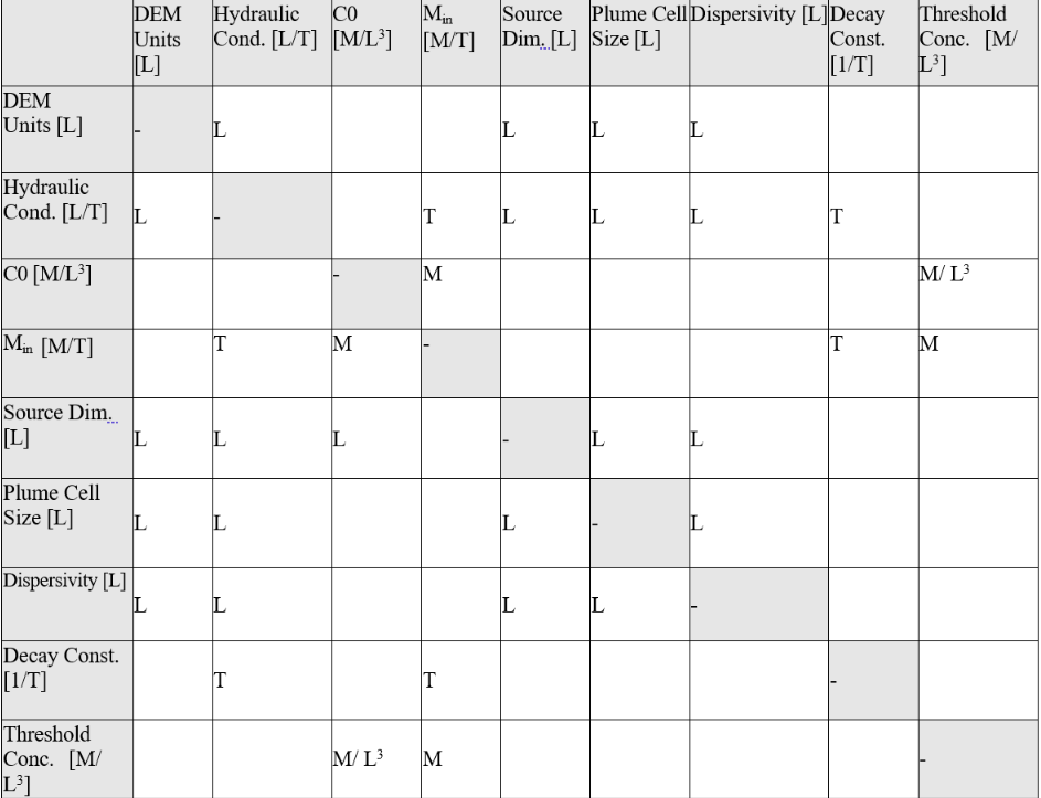
Table 8-1: Unit consistency quick reference for parameters.

Description of Modeling Data

This example focuses on the Lakeshore neighborhood of Jacksonville, Florida. In this neighborhood, houses are served by OSTDS. The Florida Department of Environmental Protection (FDEP) provides a map of OSTDS locations assumed to be at the center of the property/parcel. To generate a map of the hydraulic gradient, a DEM of the area was obtained from the National Elevation Dataset (NED) service maintained by the USGS. This DEM has a horizontal resolution of 1/3 arc seconds (approximately 10 meters). Although higher-resolution data may be available, using a higher resolution may not be appropriate because the increased detail is not well suited for hydrologic simulations (Wolock and Price, 1994). Shapefiles that contain the location information of water bodies that may be impacted were obtained for the FDEP. Groundwater flow and transport parameters used in this example are taken from the literature. This example serves for training purposes and not for realistic estimation of nitrate load in the Lakeshore neighborhood.

When using your data, the procedure for obtaining the DEM data is given in the Preparing Input Data section. Other data needed for running the software (e.g., the water body polygons) is obtainable from an appropriate database such as the National Hydrography Dataset (NHD) and FDEP.

The unprocessed DEM and water body data are provided for reference in the Examples directory in the ZIP file. For illustration purposes, this section outlines the required steps to prepare data for use in ArcNLET-Py.

Lakeshore Example Data

The Lakeshore Example, created from real-world data, allows you to model groundwater and soil interactions that produce pollution plumes and load estimates for nitrate. The Lakeshore Example exercise is designed to acclimate you to the ArcNLET-Py Python Toolbox within the ArcGIS Pro desktop environment.

Open ArcGIS Pro

1. Ensure you have completed all the steps for installing ArcGIS Pro before continuing.

   1. ArcGIS Pro must be installed, and the ArcNLET-Py repository [Download ZIP] file from GitHub must be saved on your local or network computer.

2. Open your current ArcGIS Pro Project File by double-clicking the [.aprx] file in the folder directory; for this example, the Project File is called [ArcNLET_2023_09_28.aprx].

   1. Please ensure that the [ArcNLET-Py-main.zip] file from GitHub has been extracted in a subfolder in this directory, as seen in Figure 8-1.

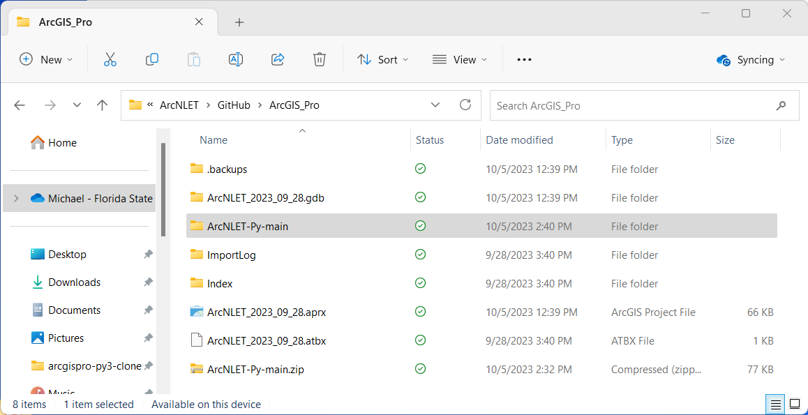
Figure 8-1: The extracted ArcNLET-Py-main folder in the Windows File Explorer.

Open ArcNLET-Py

1. Once your ArcGIS Pro Project File is open, navigate to the [Catalog Pane] or [Catalog View] as seen in Figure 8-2 and Figure 8-3. Click the expand arrow for [Folders], and you may notice there are two [ArcNLET-Py-main] folders (…\\ArcNLET-Py-main\ArcNLET-Py-main). The folder structure is due to the way GitHub extracts the repository. In the second [ArcNLET-Py-main] folder, look for the [ArcNLET] folder that contains the [ArcNLET.pyt] ArcGIS Pro Python Toolbox.

   1. You can access the ArcNLET Toolset in the [ArcNLET.pyt] toolbox by clicking the expand arrow next to the toolbox. The toolbox includes the following modules/tools: 0-Preprocessing, 1-Groundwater Flow, 2-Particle Tracking, 3-VZMOD, 4-Transport, and 5-Load Estimation.

   2. 3-VZMOD is an optional tool for modeling ammonium and nitrate, and/or phosphate decay within the Vadose Zone.

   3. Note that tools in the ArcNLET Toolset are called modules.

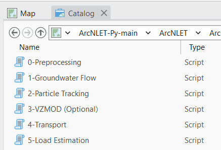
Figure 8-2: The ArcNLET-Py Python Toolset in the Catalog View in ArcGIS Pro.

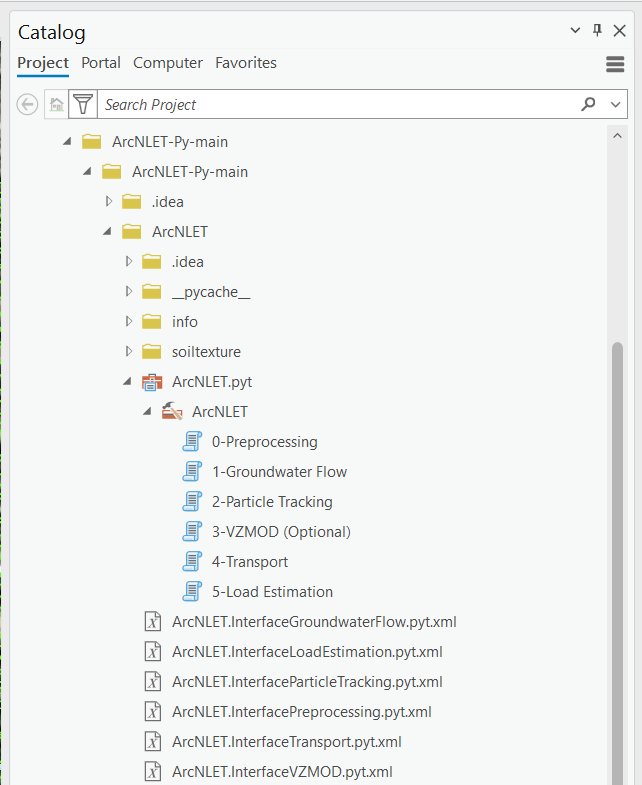
Figure 8-3: The ArcNLET-Py Python Toolset in the Catalog Pane in ArcGIS Pro.

Download and Extract Example Data

The zip file contains a fully completed model run and all processed input and output files required to generate results. The subfolder, named Examples, contains unprocessed information. This information includes unclipped and unprojected DEM and unprocessed (but clipped) water body data.

1. For this case, we use the Lakeshore Example for phosphorus, [2_lakeshore_example_phosphorus] at the following URL: https://github.com/ArcNLET-Py/ArcNLET-Py/blob/main/Examples/lakeshore_example.zip.

   1. Click the link, and the zip file should automatically download to your [Downloads] folder. You should receive a notification from your web browser when the download is completed (Figure 8-4).

   2. If the download does not begin, please check your pop-up blocker.

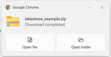
Figure 8-4: The download notification for lakeshore_example.zip.

2. Navigate to your [Downloads] folder and locate the example data in the file labeled [lakeshore_example.zip], as seen in Figure 8-5.

3. Move (Copy and Paste) the zip file to your ArcGIS Pro Project home folder where your ArcGIS Pro Project (.aprx) file was saved in Section 3.3.

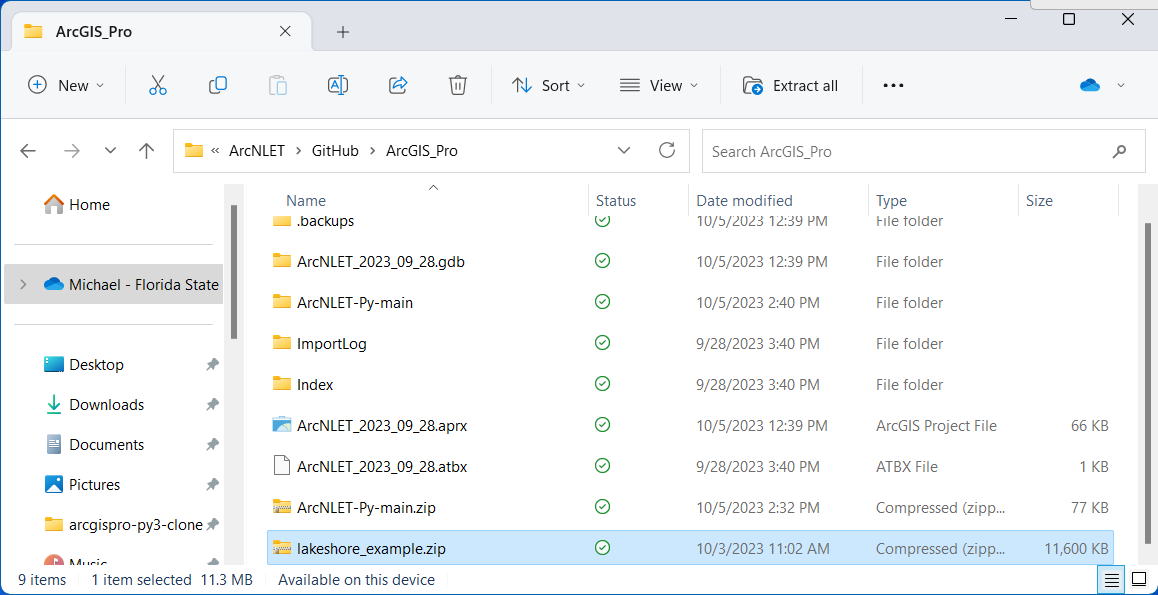
Figure 8-5: The lakeshore_example.zip file in the Windows File Explorer.

4. With the zip file in the same file directory as your ArcGIS Pro Project file, right-click the file [lakeshore_example.zip] and select [Extract All…] shown in Figure 8-6.

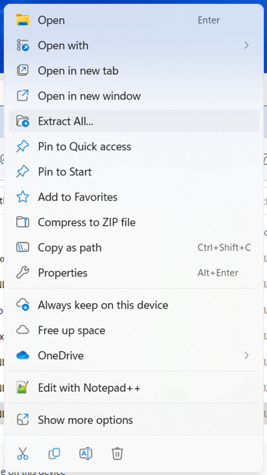
Figure 8-6: The Extract All… option in the right-click submenu.

5. The [Extract Compressed (Zipped) Folders] dialog box displays the destination for the file extraction. Please use the default setting and click [Extract], which extracts the file’s contents to a subfolder in the current directory called [lakeshore_example] (Figure 8-7).

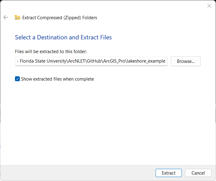
Figure 8-7: The Extract Compressed (Zipped) Folders window for ArcNLET-Py-main.zip.

6. Return to your ArcGIS Pro Project, navigate to the [Catalog View] or [Catalog Pane], right-click the icon for [Folders], and click [Refresh], as shown in Figure 8-8. Refreshing the folders updates the information and makes your newly extracted data available in ArcGIS Pro.

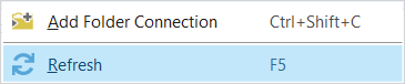
8-8: The refresh option in the right-click menu in ArcGIS Pro.Figure

7. Now, you can expand the [Folders] selection by clicking the down arrow, revealing the file connections in your ArcGIS Pro Project. Notice there are three lakeshore examples as shown in Figure 8-9. All three examples have folders for the modules used in the example, and each contain a complet set of input and output data.

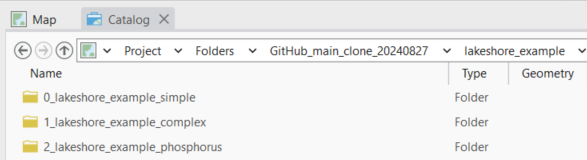
8-9: The three Lakeshore example folders.

1. [0_lakeshore_example_simple]: This is the most straight forward example that uses the least amount of modules to get nitrate load estimations. This is a great leaping off point if you are new to ArcNLET. The file contains inputs and outputs for the Groundwater Flow Module, Particle Tracking Module, Transport Module, and the Load Estimation Module.

2. [1_lakeshore_example_complex]: This example is more comprehensive and uses all five modules to estimate both ammonium and nitrate loads. It includes the 0-Preprocessing, 1-Groundwater Flow, 2-Particle Tracking, 3-VZMOD, 4-Transport, and 5-Load Estimation modules. This example provides a thorough walkthrough of each step, making it ideal for users who want to explore the full capabilities of ArcNLET for modeling complex scenarios.

3. [2_lakeshore_example_phosphorus]: This example uses all five modules to model ammonium, nitrate, and phosphate loads, providing a complete analysis of nutrient transport and load estimation. It incorporates the 0-Preprocessing, 1-Groundwater Flow, 2-Particle Tracking, 3-VZMOD, 4-Transport, and 5-Load Estimation modules. This example is ideal for users aiming to understand the impact of multiple nutrients on groundwater and surface water quality in a more detailed and complex setting.

8. Navigate to the […\lakeshore_example\2_lakeshore_example_phosphorus\…inputs] folders to see the shapefiles and raster image files needed for the exercise.

   1. Please verify that all the files were extracted correctly. You should have two additional folders: the [ArcNLET-Py-main], which contains the ArcGIS Pro Python Toolbox, and the [lakeshore_example] file folder, which contains the example data.

   2. The files needed for this exercise are shown in Figure 8-10 and are listed as follows:

      1. [study_area.shp]

         1. This shapefile defines the study area boundaries and is required for the Preprocessing Module.

      2. [lakeshore.img]

         1. The digital elevation model (DEM) of the land surface from the United States Geologic Survey (USGS) The National Map Download Client (TNM Download), used in the Groundwater Flow Module.

      3. [waterbodies.shp]

         1. The water bodies shapefile derived from the USGS TNM Download, used in the Groundwater Flow Module.

      4. [PotentialSepticTankLocations.shp]

         1. This shapefile identifies potential septic tank locations and is required for the Particle Tracking Module.

   3. Note: All other necessary inputs are derived from the operation of the ArcNLET modules. Every input and output file for all modules is available in the Inputs folders for your convenience.

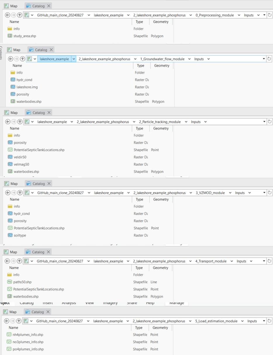
Figure 8-10: The GIS files in ArcGIS Pro for the Lakeshore example in the Catalog View.

ArcNLET-Py Toolbox

ArcNLET-Py is built to work directly in the ArcGIS Pro environment with no installation. If you are familiar with Esri Geoprocessing tools, working with the ArcNLET-Py toolsets/modules is straightforward.

ArcNLET.pyt ArcGIS Python Toolbox

In the [Catalog View] or [Catalog Pane], click the down-down arrow to expand the [ArcNLET-Py-main\ArcNLET-Py-main] and [ArcNLET] folders to expose the [ArcNLET.pyt] ArcGIS Pro Python Toolbox, as shown in Figure 8-11.

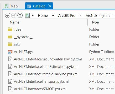
Figure 8-11: The ArcNLET-Py Python Toolbox in the Catalog View.

ArcNLET-Py ArcGIS Pro Python Toolsets

Click the drop-down arrow next to the [ArcNLET.pyt] Python Toolbox to expose the toolsets inside of the toolbox as shown in Figure 8-12. Six modules comprise the ArcNLET-Py ArcGIS Pro Python toolset, which are the Preprocessing Module (0 Preprocessing), the Groundwater Flow Module (1 Groundwater Flow), the Particle Tracking Module (2 Particle Tracking), the optional VZMOD Module (3 VZMOD (Optional)), the Transport Module (4 Transport), and the Load Estimation Module (5 Load Estimation).

Figure 8-12: The ArcNLET-Py Python Toolset in the Catalog Pane in ArcGIS Pro.

Detailed steps: - Using the Preprocessing Module for using preprocessing. - Using the Groundwater Flow Module on using groundwater flow. - Using the Particle Tracking Module for particle tracking usage. - Using the VZMOD Module for applying vertical zone modeling. - Using the Transport Module on transport modeling. - Using the Load Estimation Module for load estimation. - Visualization for visualization techniques.