1-Groundwater Flow

In traditional groundwater modeling, groundwater velocity is calculated using Darcy’s Law. Darcy’s Law requires determining the hydraulic head everywhere in the domain by solving a differential equation (heat equation) given certain initial and boundary conditions. Once the hydraulic head is known everywhere, the hydraulic gradient can be calculated, and the flow velocities can be determined using Darcy’s Law. Traditional tools are challenging to use and require field data that is not usually readily available. The task is to devise a simplified groundwater flow model that reduces data requirements and integrates into ArcGIS Pro.

Obtaining field data for calculating the hydraulic head of the surficial aquifer (either by solving a differential equation or by interpolation) is complex and resource-intensive. The approach taken by this model is to assume that the hydraulic head distribution of the surficial aquifer (e.g., the water table) is a subdued replica of the topography. A subdued replica means the shape of the water table can generally follow the shape of the overlying topography. In other words, if the topography has many peaks and dips, the water table is smoother and has fewer peaks and dips. This assumption is widely used (either explicitly or implicitly) in hydrological modeling. Topographic data is readily available through digital elevation models (DEMs). By processing a DEM, generating a subdued replica of the topography is possible, thereby reducing traditional groundwater modeling data requirements.

It is necessary to make several approximations regarding the system to use the processed DEM as a proxy for the water table. First, the system is assumed to be in a steady state. This state means that the generated water table should be considered an “average” over time. The Smoothing Factor parameter value is the number of smoothings that the user inputs. A larger number leads to a smoother DEM. A very large number (e.g., 1,000) of Smoothing Factor leads to a flat smoothed DEM. The Groundwater Flow Module also assumes that the Dupuit approximation is valid in the surficial aquifer. Under the Dupuit conditions, vertical hydraulic gradients can be ignored (i.e., flow is horizontal only, and simulating two-dimensional flow is sufficient for three-dimensional domains), and the hydraulic gradient is considered equal to the slope of the water table. Finally, flow is assumed to occur solely within the surficial aquifer. In other words, unsaturated flow, flow to or from confined aquifers, and the interactions between groundwater and surface water are not considered. Additionally, recharge is also not considered.

The mandatory outputs of the Groundwater Flow Module (Figure 1-1) are two raster datasets representing the magnitude and direction components of the groundwater flow velocity vector. The module has the optional raster outputs for hydraulic gradient and the smoothed DEM. The smoothed DEM raster can be used to calculate the depth from the bottom of the OSTDS to the water table using the optional VZMOD Module.

For a new ArcNLET-Py modeling, the Groundwater Flow Module is the first module that needs to be run. All other modules in the ArcNLET-Py toolbox depend on the groundwater velocity for their calculations. If groundwater velocity does not change in a new execution, there is no need to rerun this module. This module uses a DEM to approximate the hydraulic gradient, which is then combined with aquifer properties to calculate groundwater seepage velocity. Inputting the DEM and aquifer properties is described below.

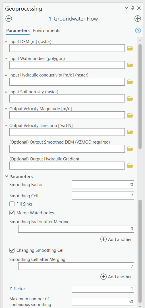
Figure 1-1: The Groundwater Flow Module in the Geoprocessing Pane.

Input Layers

• Input DEM [m] (raster): Used to generate an approximation of the water table. This input must be a raster layer (preferably in GRID format). Note that a higher resolution DEM does not necessarily give better results since a coarser DEM may better approximate the water table (Wolock and Price, 1994). This DEM is the base for all processing in this module.

• Input Water bodies (polygon): Must be a polygon-type layer. This dataset determines the locations of water bodies to which groundwater flows. This input is also used when the Fill Sinks option is selected.

• Input Hydraulic conductivity [m/d] (raster): Must be a raster layer. This input represents a map of hydraulic conductivity for the domain. The linear units of the hydraulic conductivity must be the same as the units of the DEM. For example, if the DEM has linear (ground distance) units of meters, the hydraulic conductivity must have units of meters per unit of time. The output seepage velocity magnitude has the same units as the input, i.e., L/T (length over time). It is the user’s responsibility to ensure that all units are consistent.

• Input Soil porosity (raster): It must be a raster layer. This input represents a map of soil porosity for the domain, and the soil porosity is used to calculate groundwater seepage velocity.

Options and Parameters

• Smoothing Factor: This controls the number of smoothing iterations performed on the DEM to generate a subdued replica of the topography. Higher numbers mean more smoothing and, thus, a flatter replica. As the number of iterations increases, the difference in the output from one iteration to the next becomes smaller and smaller. Values typically range between 20 and 100 depending on the specific application area. The optimum value may be determined by comparing the smoothed DEM with hydraulic head observations. The default value is 20.

• Smoothing Cell: This is the window size or neighborhood for smoothing the DEM. An odd number is recommended. The default value is 7, meaning that in a smoothing calculation, the center of the window in the DEM becomes the average of all the pixels in the 7-by-7 neighborhood around it.

• Fill Sinks: Enables or turns off sink-filling. It is helpful to enable sink-filling when the presence of sinks or pits in the DEM causes flowlines (generated by the Particle Tracking Module, see Section 2.3) to become trapped before they reach a water body. More details about filling sinks are available at https://pro.arcgis.com/en/pro-app/latest/tool-reference/spatial-analyst/how-fill-works.htm. Generally speaking, leaving sink-filling disabled (the default of ArcNLET-Py) can be advantageous, even if some pits remain after smoothing, but only if the pits do not interfere with the flow lines. As part of the sink-filling functionality, areas in the smoothed input DEM that are overlain by a water body are superimposed onto the sink-filled DEM, thereby preserving low-elevation areas in large water bodies (smaller water bodies are likely smoothed away). This superposition of the smoothed, unfilled DEM in areas where water bodies are present can be helpful in limited circumstances where sink-filling has caused the cells of the smoothed DEM immediately bordering a water body to flow in unnatural directions.

• Merge Water bodies: During the smoothing process, the elevation at water bodies often increases, which artificially decreases the control of water bodies on groundwater flow, since groundwater typically discharges to these water bodies. To address this, the original DEM where the water bodies are located can be merged with the smoothed DEM, which helps restore the influence of water bodies on groundwater flow. This merging process may be repeated several times until reasonable groundwater flow paths are obtained in the Particle Tracking Module.

  1. Smoothing Factor after Merging: After merging, additional smoothing iterations can be applied to ensure that the integration of the water bodies with the smoothed DEM results in realistic groundwater flow paths. The smoothing factor controls the number of these iterations, and adjusting it allows for fine-tuning the impact of the merging process on the flow paths.

  2. Changing Smoothing Cell: By adjusting the size of the smoothing cell, the user can control the level of detail applied during the smoothing process. Decreasing the neighborhood size can enhance the resolution of the smoothing near surface water bodies, generating more accurate gradients. This is particularly useful for guiding particles to flow into natural features like ditches, canals, and lakes rather than becoming trapped in artificial ‘gaps’ at the edge of these water features.

  3. Smoothing Cell after Merging: This parameter allows for further customization of the smoothing process after merging. By decreasing the size of the smoothing cell and merging water body elevations into the smoothed DEM, the model can better simulate the natural gradients that direct particles toward surface water bodies. This approach improves the representation of groundwater flow by creating realistic paths that lead particles into water bodies, enhancing the accuracy of flow modeling in areas with complex surface water features.

• Z-Factor: If the horizontal measurement units of the input DEM are different than the vertical units, the Z-factor value serves as a conversion factor to convert the vertical unit into the horizontal unit, which is necessary for slope calculations. For example, if the horizontal units are meters and the vertical units are feet, the z-factor is 0.3048 since one-foot equals 0.3048 meters. If the units are the same, this value should be left at the default 1. Note that the Z-Factor cannot be used to convert between two different horizontal measurement units.

Outputs

• Velocity Magnitude [m/d]: Each cell in this raster represents the magnitude of the seepage velocity in the same units as the hydraulic conductivity. The output format is a GRID raster.

• Output Velocity Direction [°wrt N]: Each cell in this raster represents the direction component of the seepage velocity in degrees clockwise from the grid north. The output format is a GRID raster.

• (Optional) Output Smoothed DEM (VZMOD required): The smoothed DEM represents the subdued replica of the topology provided by the input DEM. This DEM represents the shape of groundwater. This DEM does not represent the elevation of the groundwater. The smoothed DEM can be used as a data input in the VZMOD module.

• (Optional) Output Hydraulic Gradient: If named, it enables the output of the raster of hydraulic gradient magnitude. The output format is a GRID raster. This output is for informational purposes only (e.g., for examining the gradient values) and is not required in the other modules.

Notes

• Inputs from geodatabases are not supported at this time. All datasets must be shapefile-based.

• The input raster images (DEM elevation, hydraulic conductivity, and porosity) should ideally have the same spatial extent. Otherwise, the output raster of velocity magnitude has the extent of the smallest input raster. The direction raster has the same extent as the input DEM.

• It is recommended for the input raster datasets to have square cells since inaccuracies may be introduced in the calculations if the cells are rectangular. The user should ensure that the sizes of the cells are the same for all raster datasets.

• Units must be consistent. For example, if the values of hydraulic conductivity are in meters per day, the input DEM should also be in units of meters.

Troubleshooting

Table 1-1 lists two possible issues encountered during model execution, their possible causes, and suggested solutions. Note that the error messages may appear for reasons other than those listed. If you cannot find a solution to the issue, you can submit a [New issue] in the ArcNLET-Py GitHub repository (Issues · ArcNLET-Py/ArcNLET-Py · GitHub) as described in the GitHub instructions at Creating an issue - GitHub Docs.

Table 1-1: The Groundwater Flow Module troubleshooting guide.

Error	Cause	Solution
Raster image outputs have a solid black fill with only null or no-data values.	There might have been an error processing the data inputs.	Ensure all your data inputs are correct, in an accessible file folder, and are uncorrupted.
Empty output datasets.	An issue with the input data, an error in the file names, or ArcGIS Pro not having read/write access to input or output file locations.	Ensure all your data inputs/outputs are correct, in an accessible file folder, and are uncorrupted.