Sensitivity and Calibration
As explained in the technical manual (Rios et al., 2011), the nitrate concentration is evaluated in ArcNLET using the two-dimensional, steady-state version of the solution of Domenico (1987) for the advection-dispersion equation. It is shown in equation (16-1).
|
|
|
(16-1) |
|
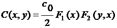
where C [ML-3] is simulated nitrate concentration at location (x,y), αx [L] is longitudinal dispersivity, αy [L] is horizontal transverse dispersivity, [L]; k [T-1] is the first order decay coefficient, v [LT−1] is groundwater seepage velocity in the longitudinal direction, Y [L] is the width of the source plane respectively, and C0 [ML-3] is the nitrate concentration at the source plane. The seepage velocity is evaluated in the groundwater flow model that uses hydraulic conductivity, porosity, and a smoothing factor to process DEM to obtain the shape of the water table. ArcNLET has seven parameters: the smoothing factor, hydraulic conductivity, porosity, longitudinal dispersivity, horizontal transverse dispersivity, first-order decay coefficient, and source nitrate concentration. Both local and global sensitivity analyses are performed to identify the parameters most critical to the simulated nitrate concentration. The local sensitivity reveals the relationships between the simulated nitrate concentration and individual parameters. The global sensitivity is more robust than the local sensitivity since it considers interactions between the parameters and the nonlinearity of the concentration concerning the parameters. For simplicity, the sensitivity to the smoothing factor, hydraulic conductivity, and porosity is not evaluated. Instead, the sensitivity to seepage velocity is calculated as a surrogate.
Local Sensitivity Analysis for Nitrate Transport
The local sensitivity is the derivative of the nitrate concentration to an individual parameter calculated for specific nominal parameter values. In this study, the nominal parameter values and their sources are as follows:
Seepage velocity: v = 0.2 m/d. This velocity is the representative value of the domains of interest.
Source plane concentration: C0 = 40 mg/L. This value is from a review article by McCray et al. (2005).
First-order decay coefficient: k = 0.008/day. This value is from a review article by McCray et al. (2005). Longitudinal dispersivity: αx = 2.113 m. This value is from the work of Davis (2000) at a vicinity site in Jacksonville, FL.
Longitudinal dispersivity: αx = 2.113 m. This value is from the work of Davis (2000) at a vicinity site in Jacksonville, FL.
Horizontal transverse dispersivity: αx = 0.234 m. This value is from the work of Davis (2000) at a vicinity site in Jacksonville, FL.
Source plane length: Y = 6m. This value is the typical length of the drain field of a septic system.
X coordinate: X = 30m. This coordinate value is arbitrarily selected for the demonstration.
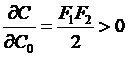
By the analytical solution, analytical expressions of the local sensitivity can be easily derived. The local sensitivity to the source plane nitrate concentration is shown in the equation (16-2).
|
 (16-2)
It suggests a positive linear relationship between the simulated nitrate concentrations and the source plane nitrate concentration. This relationship is illustrated in Figure 16-1 for two y values, the nominal parameters’ values listed above. The equation and figure show that the increase in source plane nitrate concentration increases the simulated concentration within the plume. The increase is prominent at locations closer to the plume center line (y=0m).
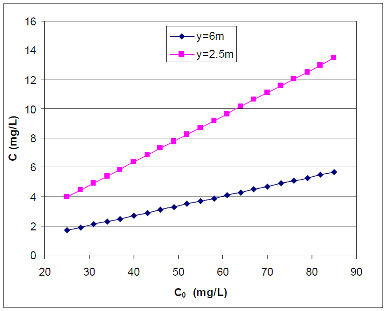
Figure 16-1: Relationship between the source plane and simulated concentrations.
For illustration, the plot shows the measured and simulated nitrate concentrations at two locations of y.
The local sensitivity to the first-order decay coefficient is shown in equation (16-3).
|
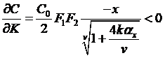 (16-3)
It suggests a negative relationship with the simulated concentration, as demonstrated in Figure 16-2. In other words, increasing the first-order decay coefficient decreases the simulated concentration within the plume. The decrease is faster at locations closer to the plume center line (y=0m).
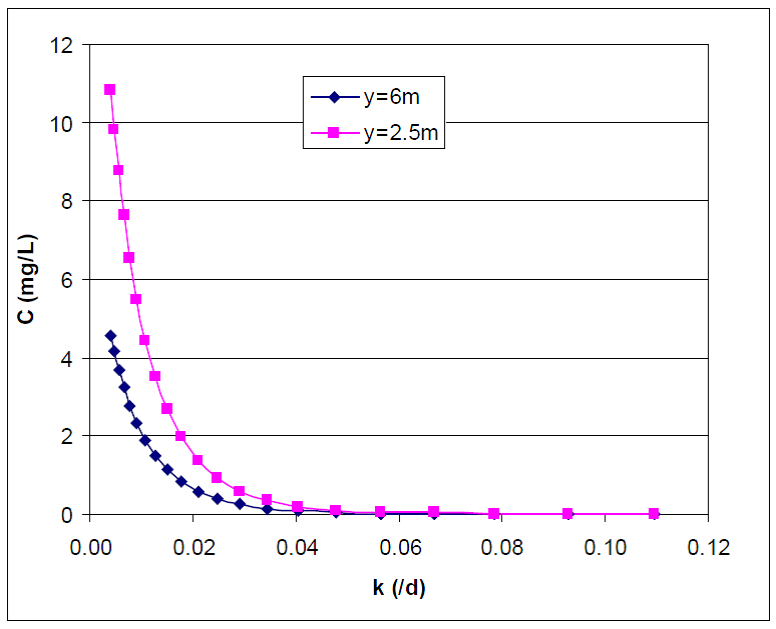
Figure 16-2: Relationship between first-order decay and concentration.
The plot illustrates the relationship between the first-order decay coefficient and simulated nitrate concentration at two locations of y.
The analytical expressions of sensitivity to the seepage velocity are shown in equation (6‑4).
|
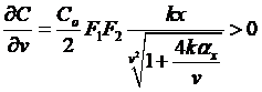 (6‑4)
(6‑4)The expression suggests a positive relationship with simulated concentration. Figure 16-3 shows that the velocity increase is associated with an increased simulated concentration within the plume. The increase is greater at locations closer to the plume center line (y=0m).
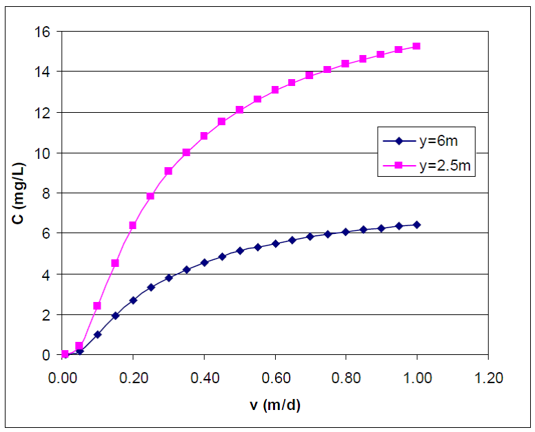
Figure 16-3: The relationship between velocity and concentration.
For illustration, the plot shows the average flow velocity and simulated nitrate concentration at two locations of y.
The analytical expression of sensitivity to the longitudinal dispersivity is shown in (16-5).
|
 (16-5)
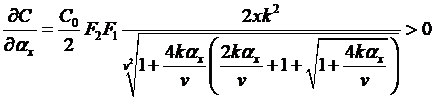
Indicates that increasing the longitudinal dispersivity causes an increase in the simulated concentration within the plume. Figure 6‑4 shows that the increase is more rapid at locations closer to the plume center line (y=0m).
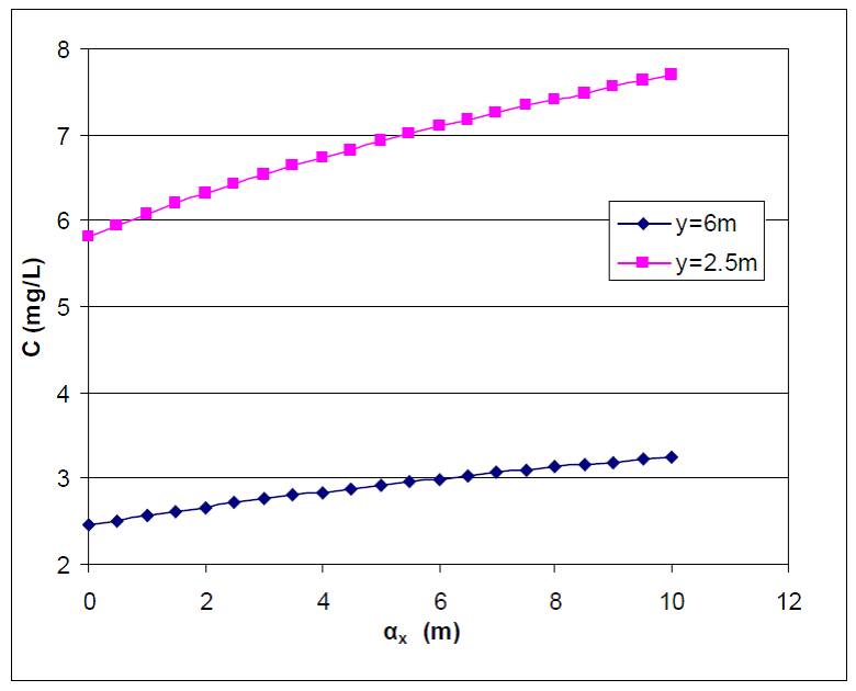
Figure 6‑4: Relationship between dispersivity and concentration.
For illustration, the plot shows the relationship between longitudinal dispersivity and simulated nitrate concentration at two locations of y.
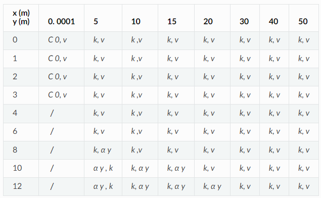
The sensitivity to the horizontal transverse dispersivity is more complicated than longitudinal. The analytical expression is shown in equation (16-6).
|
|
|
(16-6) |
|
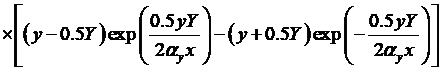
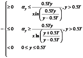
The equation above shows that the relationship between the simulated nitrate concentration and the parameter depends on the length of the source plane (Y) and the location (x and y) in the plume. In addition, there is a threshold value shown in equation (16-7).
|
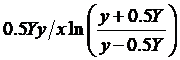 (16-7)
When the horizontal transverse dispersivity is smaller than the threshold value, the relationship is positive but becomes negative when the threshold value is exceeded. This is demonstrated in Figure 16-5.
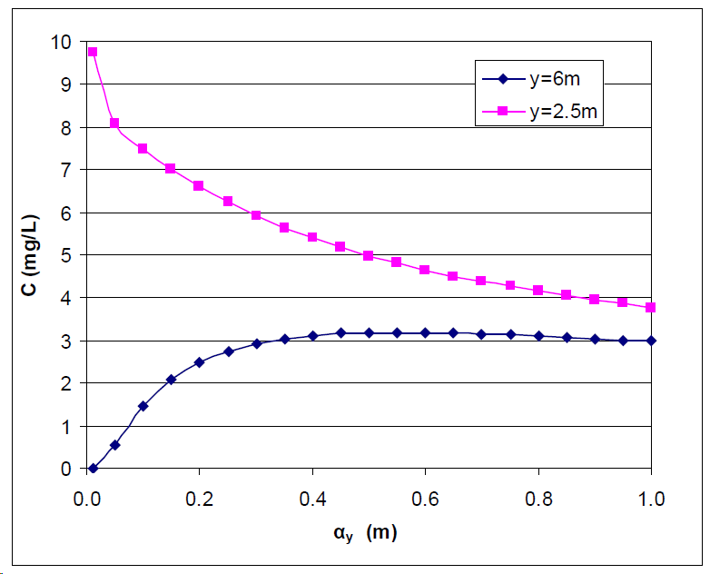
Figure 16-5: Relationship between horizontal dispersivity and concentration.
For illustration, the plot shows the relationship between horizontal transverse dispersivity and simulated nitrate concentration at two locations of y.
In summary, the local sensitivity analyses indicate that the simulated concentration is an increasing function of the source plane concentration, flow velocity, and longitude dispersivity but a decreasing function of the decay coefficient. The relationship with the horizontal transverse dispersivity depends on the parameter value and the locations where concentration is evaluated. These results are physically reasonable. For example, a large value of the decay coefficient means more denitrification and, thus, small values of simulated concentration. The relationships serve as guidelines for adjusting model parameters by trial and error to match field observations of nitrate concentration during the model calibration.
Local Sensitivity Analysis for Phosphate Transport
The main objective of this section is to analyze the effect of the phosphorus module parameters on the sensitivity of the results.
Linear Sorption Isotherm Analysis
The initial concentration: C₀ = 10 mg P/L, is used as the default value in VZMOD. Results are presented as ratios of concentration at specific depths to the initial concentration, making the specific value of the initial concentration irrelevant.
Soil type: Sand, chosen based on Florida’s conditions.
Depth to water table: Depth = 150 cm, which is the default value.
Linear distribution coefficient: k = 15.1 L/kg, based on McCray et al. (2005).
Precipitation rate: Rprecip = 0.002 1/day, referenced from Zhou et al. (2023) and Müller and Bünemann (2014).
In this study, the ratios of concentrations at the full depth and half-depth to the initial concentration were used as the y-values. Various precipitation rates and linear distribution coefficients were applied to examine their relationship with these ratios. Results are presented in Figure 16-6, showing negative correlations between the concentration ratios and parameters. Higher precipitation rates and sorption coefficients result in less phosphorus leaching. The parameters can be adjusted based on the ranges shown in Figure 16-6. Site-specific calibration is highly recommended for phosphorus modeling.

Figure 16-6: Relationships between C/C0 and (a) precipitation rate, and (b) linear distribution coefficient for the linear sorption isotherm.
Langmuir Sorption Isotherm Analysis
The Langmuir sorption isotherm was also analyzed with initial conditions similar to those used previously:
Precipitation rate: Rprecip = 0.002 1/day, consistent with Zhou et al. (2023) and Müller and Bünemann (2014).
Langmuir coefficient: K = 0.2 L/mg, values from Zhou et al. (2023) and McGechan and Lewis (2002).
Maximum sorption capacity: Qmax = 237 mg P/kg, referenced from McCray et al. (2005).
Various precipitation rates, Langmuir coefficients, and maximum sorption capacity were applied to examine their relationship with concentration ratios. Results are shown in Figures 16-7 and 16-8. Site-specific calibration is recommended for phosphorus modeling.
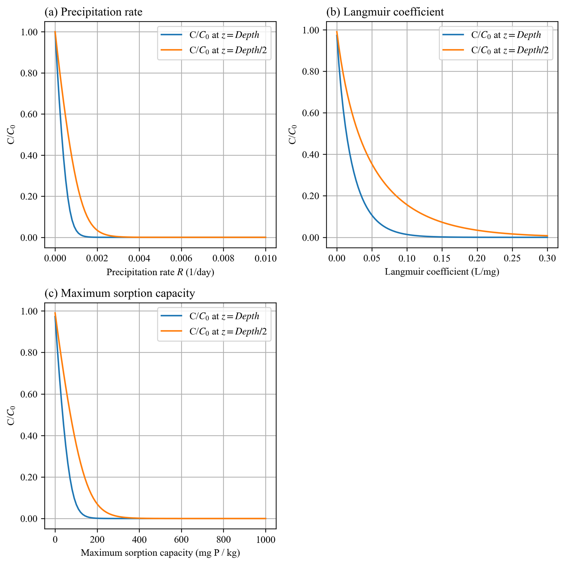
Figure 16-7: Relationships between C/C0 and (a) precipitation rate, (b) Langmuir coefficient, and (c) maximum sorption capacity for the Langmuir sorption isotherm.
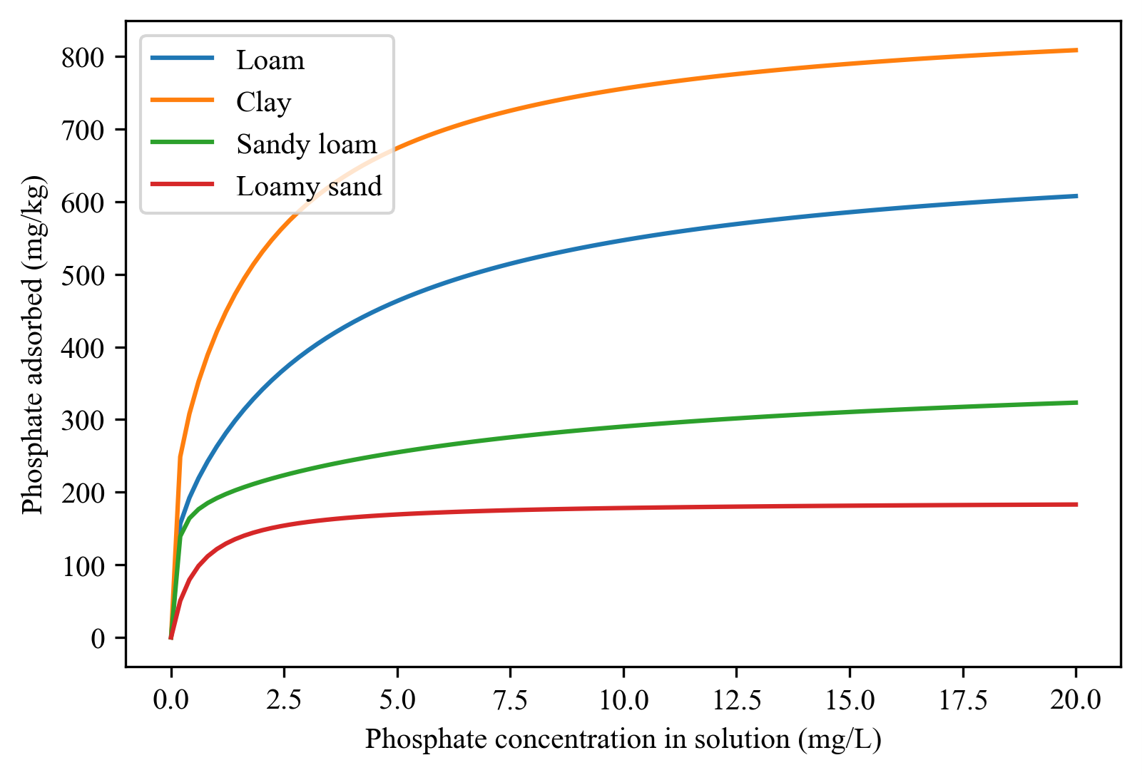
Figure 16-8: Various sorption isotherms for different soil types with the data given by McGechan (2002).
Sensitivity in Groundwater
Nominal parameter values for groundwater include:
Seepage velocity: v = 0.2 m/d.
Longitudinal dispersivity: αx = 2.113 m (Davis, 2000).
Horizontal transverse dispersivity: αy = 0.234 m (Davis, 2000).
Source plane length: Y = 6 m.
Bulk density: ρ = 1.42 g/cm³.
Porosity: θ = 0.4 cm³/cm³.
Linear distribution coefficient: k = 15.1 L/kg (McCray et al., 2005).
Precipitation rate: Rprecip = 0.002 1/day.
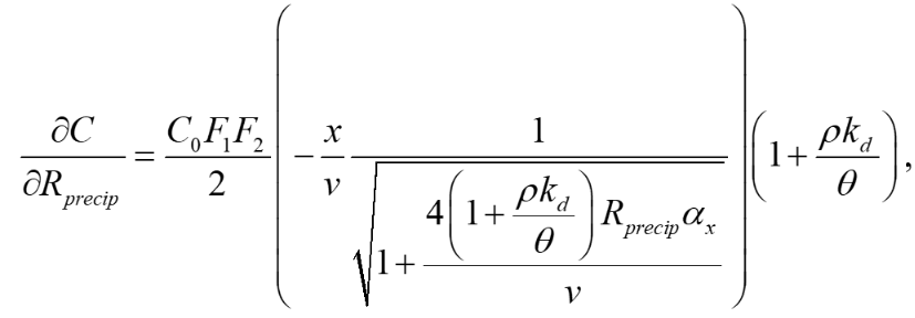
The analytical expressions of sensitivity to precipitation rate and linear distribution coefficient are shown in equations (17) and (18). Increasing these parameters leads to a decrease in the simulated concentration within the plume.
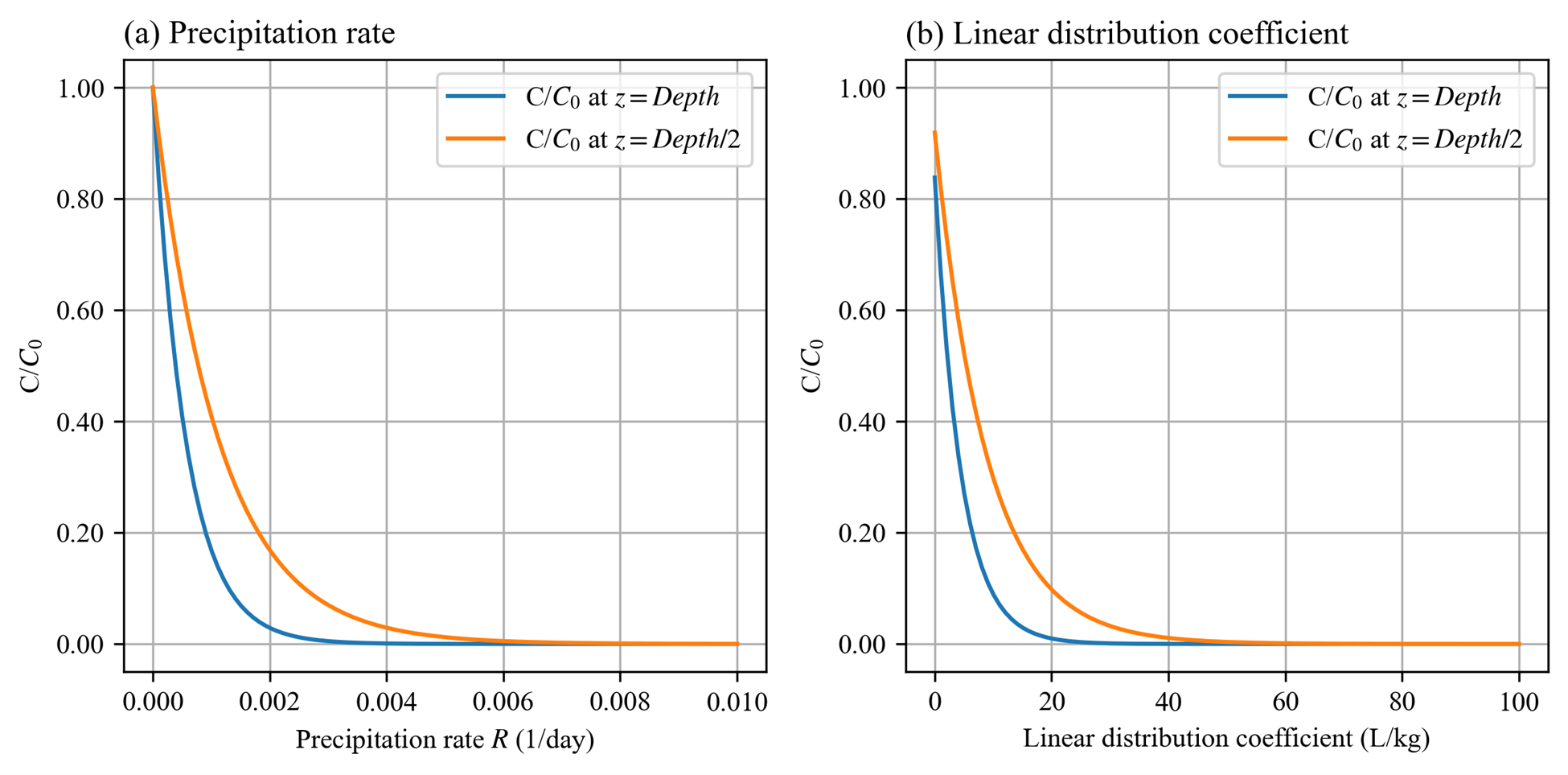
Figure 16-9: Relationships between C/C0 and (a) precipitation rate, and (b) linear distribution coefficient for linear sorption in groundwater.
Sensitivity in VZMOD
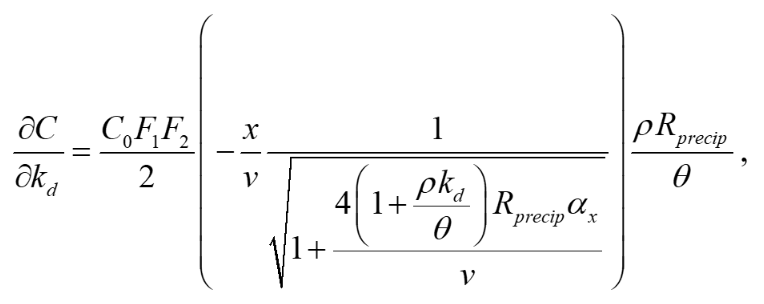
VZMOD, being a steady-state model, adopts smaller values than those used in Zhou et al. (2023). The analytical expressions of sensitivity to the precipitation rate and linear distribution coefficient are represented by Equations (16-8) and (16-9):
|
(16-8) |
|---|---|
|
(16-9) |
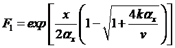
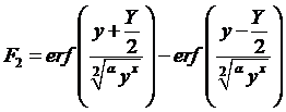
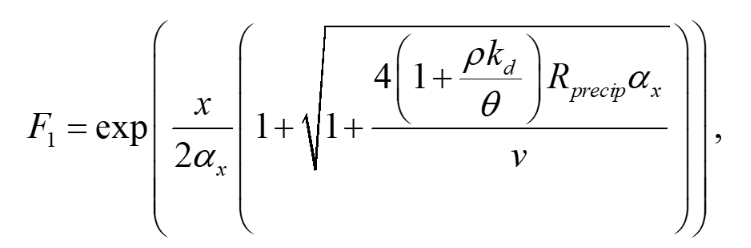
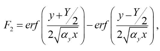
Where F1 and F2 are calculated as follows:
|
(16-10) |
|---|---|
|
(16-11) |
These expressions suggest negative relationships with the simulated concentration. Specifically, increasing the precipitation rate and linear distribution coefficient results in a decrease in the simulated concentration within the plume, with a more rapid decline observed at locations closer to the plume centerline (y = 0 m).
Summary
The sensitivity analyses indicate that phosphorus sorption is significantly influenced by factors such as Fe concentration, total organic carbon concentration, pH, and others. These findings suggest that site-specific calibration is essential for accurate phosphorus modeling.
Model Calibration
Generally speaking, model calibration matches the simulated nitrate and phosphorus concentrations to observed values by adjusting model parameters. Due to the lack of comprehensive characterization data, model calibration in this study is necessary.
For nitrate, calibration begins with adjusting parameters like hydraulic conductivity, porosity, dispersivities, and decay coefficients to match observed concentrations. Phosphorus modeling also involves fine-tuning precipitation rates, sorption coefficients, and other related parameters.
Note
Site-specific calibration is recommended to enhance the accuracy of both nitrate and phosphorus modeling due to the varying influence of site conditions on sorption processes.
Generally speaking, model calibration matches the simulated nitrate concentration to the observed ones by adjusting the model parameters. Model calibration in this study is necessary due to the lack of characterization data for describing the hydrogeologic conditions of the modeling domains. For example, no other parameter measure is available except for the hydraulic conductivity and porosity downloaded from the SSURGO database. The only site-specific measurements are the particulate organic carbon (POC) content collected from the Eggleston Heights and Julington Creek neighborhoods at the top 1.5 m of the saturated zone. The data shows that the average POC content is 0.35% and 1.08% in the Eggleston Heights and Julington Creek neighborhoods. Anderson (1998) states that the denitrification rate is positively correlated with POC content. The higher POC content in the Julington Creek area suggests a higher denitrification rate. This data is taken as prior information for the model calibration.
The trial-and-error model calibration starts from the Eggleston Height neighborhood by evaluating nitrate concentration in the modeling domains using the smoothing factor of 60, heterogeneous hydraulic conductivity and porosity downloaded from the SSURGO database, longitude dispersivity αx of 2.113 m (Davis 2000), αy of 0.234 m (Davis 2000), C0 of 40 mg/L (McCray et al. 2005), and first-order decay coefficient k of 0.025/d (McCray et al. 2005). The most sensitive parameters identified in the sensitivity analyses are subsequently adjusted to obtain an improved fit between the simulated and observed nitrate concentration. The sensitivity to seepage velocity is reflected by adjusting hydraulic conductivity because it plays the most critical role in determining the velocity’s magnitude.
The detailed procedure of model calibration within ArcNLET is as follows:
Calibrate the flow model by adjusting the smoothing factor and using the mean hydraulic head observations at the monitoring wells as the calibrated targets. Since ArcNLET does not simulate hydraulic head but hydraulic gradient, the goal of adjusting the smoothing factor is to obtain a linear relationship between the smoothed DEM (which is an intermediate output layer of the Groundwater Flow Module, described in detail in the user’s manual) and the calibration targets values at the observation wells. The slope of the linear relationship must be close to 1.0 so that the shape of the smoothed DEM mimics the shape of the water table. Hydraulic conductivity is not calibrated in this step unless observations of groundwater velocity are available.
Calibrate the transport model using trial and error by adjusting the first-order decay coefficient, hydraulic conductivity, dispersivities, and source concentration. The calibration goal is to match the simulated nitrate concentration to the mean observations at the monitoring wells. Due to the complex nature of nitrate transport and the simplicity of the model behind ArcNLET, it is not likely that the match is achieved at all the wells. A reasonable expectation is that the simulated nitrate concentration falls in the inter-quartile range or maximum and minimum observations at each well. Given that multiple septic systems can impact nitrate concentration at a monitoring well, the global sensitivity analysis results are essential guidelines to adjust different parameters for different septic systems. Using homogenous values of the first-order decay coefficient, dispersivities, and source concentration is recommended because they may be considered representative values of the modeling domain. Adjusting the hydraulic conductivity within the high and low values given in the soil survey data is recommended.
Based on our experience, the model calibration for the flow model is relatively easy. In contrast, the calibration of the transport model may be time-consuming and require a solid understanding of the nitrate transport from the hydrogeologic point of view.